User’s Guide¶

This manual provides reference documentation to SfePy from a user’s perspective.

Running a Simulation ¶

The following should be run in the top-level directory of the SfePy source tree after installing the sfepy package. See Installation for installation instructions.

Running Tests ¶

The tests are based on pytest and can be run using:

python -c "import sfepy; sfepy.test()"

See Testing Installation for additional information.

Computations and Examples ¶

Most of the example problems in the sfepy/examples directory can be computed by the sfepy-run command. Additional (stand-alone) examples can be run directly, e.g.:

python sfepy/examples/large_deformation/compare_elastic_materials.py

Common Tasks ¶

Run a simulation:

sfepy-run sfepy/examples/diffusion/poisson_short_syntax.py
sfepy-run sfepy/examples/diffusion/poisson_short_syntax.py -o some_results # -> produces some_results.vtk

Print available terms:
```
sfepy-run --list=terms
```

Run a simulation and also save Dirichlet boundary conditions:

sfepy-run --save-ebc sfepy/examples/diffusion/poisson_short_syntax.py # -> produces an additional .vtk file with BC visualization

Use a restart file to continue an interrupted simulation:
- Warning: This feature is preliminary and does not support terms with internal state.
- Run:
```
sfepy-run sfepy/examples/large_deformation/balloon.py --save-restart=-1
```
  and break the computation after a while (hit Ctrl-C). The mode --save-restart=-1 is currently the only supported mode. It saves a restart file for each time step, and only the last computed time step restart file is kept.
- A file named 'unit_ball.restart-??.h5' should be created, where '??' indicates the last stored time step. Let us assume it is 'unit_ball.restart-04.h5', i.e. the fifth step.
- Restart the simulation by:
```
sfepy-run sfepy/examples/large_deformation/balloon.py --load-restart=unit_ball.restart-04.h5
```
  The simulation should continue from the next time step. Verify that by running:
```
sfepy-run sfepy/examples/large_deformation/balloon.py
```
  and compare the residuals printed in the corresponding time steps.

Visualization of Results ¶

Quick visualisation of the SfePy results can be done by sfepy.scripts.resview.py command, which uses PyVista visualization toolkit (need to be installed).

For example, results of a stationary Navier-Stokes flow simulation:

sfepy-run sfepy/examples/navier_stokes/navier_stokes.py -o navier_stokes

can be viewed using:

sfepy-view navier_stokes.vtk

produces:

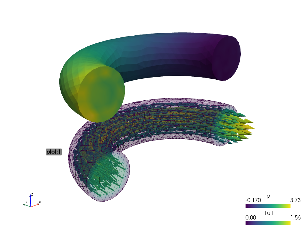
Using:

sfepy-view navier_stokes.vtk -f p:i5:p0 p:e:o.2:p0 u:t1000:p1 u:o.2:p1

the output is split into plots plot:0 and plot:1, where these plots contain:

plot:0: field p, 5 isosurfaces, mesh edges switched on, the surface opacity set to 0.2;
plot:1: vector field u streamlines, the surface opacity set to 0.2;

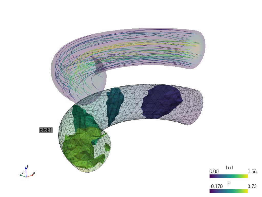
The actual camera position can be printed by pressing the ‘c’ key. The above figures use the following values:

--camera-position="-0.236731,-0.352216,0.237044,0.094458,0.0292563,0.0385116,0.266969,0.252278,0.930099"

The argument -o filename.png takes the screenshot of the produced view:

sfepy-view navier_stokes.vtk -o image.png

Problem Description File ¶

Here we discuss the basic items that users have to specify in their input files. For complete examples, see the problem description files in the sfepy/examples/ directory of SfePy.

Besides the short syntax described below there is (due to history) also a long syntax which is explained in Problem Description File - Long Syntax. The short and long syntax can be mixed together in one description file.

FE Mesh ¶

A FE mesh defining a domain geometry can be stored in several formats:

legacy VTK (.vtk)
custom HDF5 file (.h5)
medit mesh file (.mesh)
tetgen mesh files (.node, .ele)
comsol text mesh file (.txt)
abaqus text mesh file (.inp)
avs-ucd text mesh file (.inp)
hypermesh text mesh file (.hmascii)
hermes3d mesh file (.mesh3d)
nastran text mesh file (.bdf)
gambit neutral text mesh file (.neu)
salome/pythonocc med binary mesh file (.med)

Example:

filename_mesh = 'meshes/3d/cylinder.vtk'

The VTK and HDF5 formats can be used for storing the results. The format can be selected in options, see Miscellaneous.

The following geometry elements are supported:

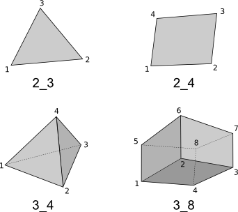
Note the orientation of the vertices matters, the figure displays the correct orientation when interpreted in a right-handed coordinate system.

Regions ¶

Regions serve to select a certain part of the computational domain using topological entities of the FE mesh. They are used to define the boundary conditions, the domains of terms and materials etc.

Let us denote D the maximal dimension of topological entities. For volume meshes it is also the dimension of space the domain is embedded in. Then the following topological entities can be defined on the mesh (notation follows [Logg2012]):

[Logg2012]

Logg: Efficient Representation of Computational Meshes. 2012

topological entity	dimension	co-dimension
vertex	0	D
edge	1	D - 1
face	2	D - 2
facet	D - 1	1
cell	D	0

If D = 2, faces are not defined and facets are edges. If D = 3, facets are faces.

Following the above definitions, a region can be of different kind:

cell, facet, face, edge, vertex - entities of higher dimension are not included.
cell_only, facet_only, face_only, edge_only, vertex_only - only the specified entities are included, other entities are empty sets, so that set-like operators still work, see below.
The cell kind is the most general and should be used with cell terms. It is also the default if the kind is not specified in region definition.
The facet kind (same as edge in 2D and face in 3D) is to be used with boundary (facet integral) terms.
The vertex (same as vertex_only) kind can be used with point-wise defined terms (e.g. point loads).

The kinds allow a clear distinction between regions of different purpose (cell integration domains, facet domains, etc.) and could be used to lower memory usage.

A region definition involves topological entity selections combined with set-like operators. The set-like operators can result in intermediate regions that have the cell kind. The desired kind is set to the final region, removing unneeded entities. Most entity selectors are defined in terms of vertices and cells - the other entities are computed as needed.

Topological Entity Selection ¶

topological entity selection	explanation
`all`	all entities of the mesh
`vertices of surface`	surface of the mesh
`vertices of group <integer>`	vertices of given group
`vertices of set <str>`	vertices of a given named vertex set [2]
`vertices in <expr>`	vertices given by an expression [3]
`vertices by <function>`	vertices given by a function of coordinates [4]
`vertex <id>[, <id>, ...]`	vertices given by their ids
`vertex in r.<name of another region>`	any single vertex in the given region
`cells of group <integer>`	cells of given group
`cells by <efunction>`	cells given by a function of coordinates [5]
`cell <id>[, <id>, ...]`,	cells given by their ids
`copy r.<name of another region>`	a copy of the given region
`r.<name of another region>`	a reference to the given region

topological entity selection footnotes

set-like operator	explanation
`+v`	vertex union
`+e`	edge union
`+f`	face union
`+s`	facet union
`+c`	cell union
`-v`	vertex difference
`-e`	edge difference
`-f`	face difference
`-s`	facet difference
`-c`	cell difference
`*v`	vertex intersection
`*e`	edge intersection
`*f`	face intersection
`*s`	facet intersection
`*c`	cell intersection

Region Definition Syntax ¶

Regions are defined by the following Python dictionary:

regions = {
    <name> : (<selection>, [<kind>], [<parent>], [{<misc. options>}]),
}

or:

regions = {
    <name> : <selection>,
}

Example definitions:

regions = {
    'Omega' : 'all',
    'Right' : ('vertices in (x > 0.99)', 'facet'),
    'Gamma1' : ("""(cells of group 1 *v cells of group 2)
                   +v r.Right""", 'facet', 'Omega'),
    'Omega_B' : 'vertices by get_ball',
}

The Omega_B region illustrates the selection by a function (see Topological Entity Selection). In this example, the function is:

import numpy as nm

def get_ball(coors, domain=None):
    x, y, z = coors[:, 0], coors[:, 1], coors[:, 2]

    r = nm.sqrt(x**2 + y**2 + z**2)
    flag = nm.where((r < 0.1))[0]

    return flag

The function needs to be registered in Functions:

functions = {
    'get_ball' : (get_ball,),
}

The mirror region can be defined explicitly as:

regions = {
  'Top': ('r.Y *v r.Surf1', 'facet', 'Y', {'mirror_region': 'Bottom'}),
  'Bottom': ('r.Y *v r.Surf2', 'facet', 'Y', {'mirror_region': 'Top'}),
}

Fields ¶

Fields correspond to FE spaces:

fields = {
    <name> : (<data_type>, <shape>, <region_name>, <approx_order>,
    [<space>, <poly_space_basis>])
}

where

<data_type> is a numpy type (float64 or complex128) or ‘real’ or ‘complex’
<shape> is the number of DOFs per node: 1 or (1,) or ‘scalar’, space dimension (2, or (2,) or 3 or (3,)) or ‘vector’; it can be other positive integer than just 1, 2, or 3
<region_name> is the name of region where the field is defined
<approx_order> is the FE approximation order, e.g. 0, 1, 2, ‘1B’ (1 with bubble)
<space> is the function space
<poly_space_basis> is the basis of the FE (usually polynomial) space

Example: scalar P1 elements in 2D on a region Omega:

fields = {
    'temperature' : ('real', 1, 'Omega', 1),
}

The following approximation orders can be used:

simplex elements: 1, 2, ‘1B’, ‘2B’

tensor product elements: 0, 1, ‘1B’

Optional bubble function enrichment is marked by ‘B’.

The implemented combinations of spaces and bases are listed below, the space column corresponds to <space>, the basis column to <poly_space_basis> and region type to the field region type.

Fields¶
space	basis	region kind	description
H1	bernstein	`cell`, `facet`	Bernstein basis approximation with positive-only basis function values.
H1	iga	`cell`	Bezier extraction based NURBS approximation for isogeometric analysis.
H1	lagrange	`cell`, `facet`	Lagrange basis nodal approximation.
H1	lagrange_discontinuous	`cell`	The C0 constant-per-cell approximation.
H1	lobatto	`cell`	Hierarchical basis approximation with Lobatto polynomials.
H1	sem	`cell`, `facet`	Spectral element method approximation.
H1	serendipity	`cell`, `facet`	Lagrange basis nodal serendipity approximation with order <= 3.
H1	shell10x	`cell`	The approximation for the shell10x element.
L2	constant	`cell`, `facet`	The L2 constant-in-a-region approximation.
DG	legendre_discontinuous	`cell`	Discontinuous Galerkin method approximation with Legendre basis.

Variables ¶

Variables use the FE approximation given by the specified field:

variables = {
    <name> : (<kind>, <field_name>, <spec>, [<history>])
}

where

<kind> - ‘unknown field’, ‘test field’ or ‘parameter field’
<spec> - in case of: primary variable - order in the global vector of unknowns, dual variable - name of primary variable
<history> - number of time steps to remember prior to current step

Example:

variables = {
    't' : ('unknown field', 'temperature', 0, 1),
    's' : ('test field', 'temperature', 't'),
}

Integrals ¶

Define the integral type and quadrature rule. This keyword is optional, as the integration orders can be specified directly in equations (see below):

integrals = {
    <name> : <order>
}

where

<name> - the integral name - it has to begin with ‘i’!
<order> - the order of polynomials to integrate, or ‘custom’ for integrals with explicitly given values and weights

Example:

import numpy as nm
N = 2
integrals = {
    'i1' : 2,
    'i2' : ('custom', zip(nm.linspace( 1e-10, 0.5, N ),
                          nm.linspace( 1e-10, 0.5, N )),
            [1./N] * N),
}

Essential Boundary Conditions and Constraints ¶

The essential boundary conditions set values of DOFs in some regions, while the constraints constrain or transform values of DOFs in some regions.

Dirichlet Boundary Conditions ¶

The Dirichlet, or essential, boundary conditions apply in a given region given by its name, and, optionally, in selected times. The times can be given either using a list of tuples (t0, t1) making the condition active for t0 <= t < t1, or by a name of a function taking the time argument and returning True or False depending on whether the condition is active at the given time or not.

Dirichlet (essential) boundary conditions:

ebcs = {
    <name> : (<region_name>, [<times_specification>,]
              {<dof_specification> : <value>[,
               <dof_specification> : <value>, ...]})
}

Example:

ebcs = {
    'u1' : ('Left', {'u.all' : 0.0}),
    'u2' : ('Right', [(0.0, 1.0)], {'u.0' : 0.1}),
    'phi' : ('Surface', {'phi.all' : 0.0}),
    'u_yz' : ('Gamma', {'u.[1,2]' : 'rotate_yz'}),
}

The u_yz condition illustrates calculating the condition value by a function. In this example, it is a function of coordinates coors of region nodes:

import numpy as nm

def rotate_yz(ts, coor, **kwargs):
    from sfepy.linalg import rotation_matrix2d

    vec = coor[:,1:3] - centre

    angle = 10.0 * ts.step

    mtx = rotation_matrix2d(angle)
    vec_rotated = nm.dot(vec, mtx)

    displacement = vec_rotated - vec

    return displacement

The function needs to be registered in Functions:

functions = {
    'rotate_yz' : (rotate_yz,),
}

Periodic Boundary Conditions ¶

The periodic boundary conditions tie DOFs of a single variable in two regions that have matching nodes. Can be used with functions in sfepy.discrete.fem.periodic.

Periodic boundary conditions:

epbcs = {
    <name> : ((<region1_name>, <region2_name>), [<times_specification>,]
              {<dof_specification> : <dof_specification>[,
               <dof_specification> : <dof_specification>, ...]},
              <match_function_name>)
}

Example:

epbcs = {
    'up1' : (('Left', 'Right'), {'u.all' : 'u.all', 'p.0' : 'p.0'},
             'match_y_line'),
}

Linear Combination Boundary Conditions ¶

The linear combination boundary conditions (LCBCs) are more general than the Dirichlet BCs or periodic BCs. They can be used to substitute one set of DOFs in a region by another set of DOFs, possibly in another region and of another variable. The LCBCs can be used only in FEM with nodal (Lagrange) basis.

Available LCBC kinds:

'rigid' - in linear elasticity problems, a region moves as a rigid body;
'no_penetration' - in flow problems, the velocity vector is constrained to the plane tangent to the surface;
'normal_direction' - the velocity vector is constrained to the normal direction;
'edge_direction' - the velocity vector is constrained to the mesh edge direction;
'integral_mean_value' - all DOFs in a region are summed to a single new DOF;
'shifted_periodic' - generalized periodic BCs that work with two different variables and can have a non-zero mutual shift;
'match_dofs' - tie DOFs of two fields.

Only the 'shifted_periodic' LCBC needs the second region and the DOF mapping function, see below.

Linear combination boundary conditions:

lcbcs = {
    'shifted' : (('Left', 'Right'),
                 {'u1.all' : 'u2.all'},
                 'match_y_line', 'shifted_periodic',
                 'get_shift'),
    'mean' : ('Middle', {'u1.all' : None}, None, 'integral_mean_value'),
}

Initial Conditions ¶

Initial conditions are applied prior to the boundary conditions - no special care must be used for the boundary dofs:

ics = {
    <name> : (<region_name>, {<dof_specification> : <value>[,
                              <dof_specification> : <value>, ...]},...)
}

Example:

ics = {
    'ic' : ('Omega', {'T.0' : 5.0}),
}

Materials ¶

Materials are used to define constitutive parameters (e.g. stiffness, permeability, or viscosity), and other non-field arguments of terms (e.g. known traction or volume forces). Depending on a particular term, the parameters can be constants, functions defined over FE mesh nodes, functions defined in the elements, etc.

Example:

material = {
    'm' : ({'val' : [0.0, -1.0, 0.0]},),
    'm2' : 'get_pars',
    'm3' : (None, 'get_pars'), # Same as the above line.
}

Example: different material parameters in regions ‘Yc’, ‘Ym’:

from sfepy.mechanics.matcoefs import stiffness_from_youngpoisson
dim = 3
materials = {
    'mat' : ({'D' : {
        'Ym': stiffness_from_youngpoisson(dim, 7.0e9, 0.4),
        'Yc': stiffness_from_youngpoisson(dim, 70.0e9, 0.2)}
    },),
}

Defining Material Parameters by Functions ¶

The functions for defining material parameters can work in two modes, distinguished by the mode argument. The two modes are ‘qp’ and ‘special’. The first mode is used for usual functions that define parameters in quadrature points (hence ‘qp’), while the second one can be used for special values like various flags.

The shape and type of data returned in the ‘special’ mode can be arbitrary (depending on the term used). On the other hand, in the ‘qp’ mode all the data have to be numpy float64 arrays with shape (n_coor, n_row, n_col), where n_coor is the number of quadrature points given by the coors argument, n_coor = coors.shape[0], and (n_row, n_col) is the shape of a material parameter in each quadrature point. For example, for scalar parameters, the shape is (n_coor, 1, 1). The shape is determined by each term.

Example:

def get_pars(ts, coors, mode=None, **kwargs):
    if mode == 'qp':
        val = coors[:,0]
        val.shape = (coors.shape[0], 1, 1)

        return {'x_coor' : val}

The function needs to be registered in Functions:

functions = {
    'get_pars' : (get_pars,),
}

If a material parameter has the same value in all quadrature points, than it is not necessary to repeat the constant and the array can be with shape (1, n_row, n_col).

Equations and Terms ¶

Equations can be built by combining terms listed in Term Table.

Examples ¶

Laplace equation, named integral:

equations = {
    'Temperature' : """dw_laplace.i.Omega( coef.val, s, t ) = 0"""
}

Laplace equation, simplified integral given by order:

equations = {
    'Temperature' : """dw_laplace.2.Omega( coef.val, s, t ) = 0"""
}

Laplace equation, automatic integration order (not implemented yet!):

equations = {
    'Temperature' : """dw_laplace.a.Omega( coef.val, s, t ) = 0"""
}

Navier-Stokes equations:

equations = {
    'balance' :
    """+ dw_div_grad.i2.Omega( fluid.viscosity, v, u )
       + dw_convect.i2.Omega( v, u )
       - dw_stokes.i1.Omega( v, p ) = 0""",
    'incompressibility' :
    """dw_stokes.i1.Omega( u, q ) = 0""",
}

Configuring Solvers ¶

In SfePy, a non-linear solver has to be specified even when solving a linear problem. The linear problem is/should be then solved in one iteration of the nonlinear solver.

Linear and nonlinear solver:

solvers = {
    'ls' : ('ls.scipy_direct', {}),
    'newton' : ('nls.newton',
                {'i_max'   : 1}),
}

Solver selection:

options = {
    'nls' : 'newton',
    'ls' : 'ls',
}

For the case that a chosen linear solver is not available, it is possible to define the fallback option of the chosen solver which specifies a possible alternative:

solvers = {
    'ls': ('ls.mumps', {'fallback': 'ls2'}),
    'ls2': ('ls.scipy_umfpack', {}),
    'newton': ('nls.newton', {
        'i_max'      : 1,
        'eps_a'      : 1e-10,
    }),
}

Another possibility is to use a “virtual” solver that ensures an automatic selection of an available solver, see Virtual Linear Solvers with Automatic Selection.

Functions ¶

Functions are a way of customizing SfePy behavior. They make it possible to define material properties, boundary conditions, parametric sweeps, and other items in an arbitrary manner. Functions are normal Python functions declared in the Problem Definition file, so they can invoke the full power of Python. In order for SfePy to make use of the functions, they must be declared using the function keyword. See the examples below, and also the corresponding sections above.

Examples ¶

See sfepy/examples/diffusion/poisson_functions.py for a complete problem description file demonstrating how to use different kinds of functions.

functions for defining regions:

def get_circle(coors, domain=None):
    r = nm.sqrt(coors[:,0]**2.0 + coors[:,1]**2.0)
    return nm.where(r < 0.2)[0]

functions = {
    'get_circle' : (get_circle,),
}

functions for defining boundary conditions:

def get_p_edge(ts, coors, bc=None, problem=None):
    if bc.name == 'p_left':
        return nm.sin(nm.pi * coors[:,1])
    else:
        return nm.cos(nm.pi * coors[:,1])

functions = {
    'get_p_edge' : (get_p_edge,),
}

ebcs = {
    'p' : ('Gamma', {'p.0' : 'get_p_edge'}),
}

The values can be given by a function of time, coordinates and possibly other data, for example:

ebcs = {
    'f1' : ('Gamma1', {'u.0' : 'get_ebc_x'}),
    'f2' : ('Gamma2', {'u.all' : 'get_ebc_all'}),
}

def get_ebc_x(coors, amplitude):
    z = coors[:, 2]
    val = amplitude * nm.sin(z * 2.0 * nm.pi)
    return val

def get_ebc_all(ts, coors):
    val = ts.step * coors
    return val

functions = {
    'get_ebc_x' : (lambda ts, coors, bc, problem, **kwargs:
                   get_ebc_x(coors, 5.0),),
    'get_ebc_all' : (lambda ts, coors, bc, problem, **kwargs:
                     get_ebc_all(ts, coors),),
}

Note that when setting more than one component as in get_ebc_all() above, the function should return either an array of shape (coors.shape[0], n_components), or the same array flattened to 1D row-by-row (i.e. node-by-node), where n_components corresponds to the number of components in the boundary condition definition. For example, with ‘u.[0, 1]’, n_components is 2.

function for defining usual material parameters:

def get_pars(ts, coors, mode=None, **kwargs):
    if mode == 'qp':
        val = coors[:,0]
        val.shape = (coors.shape[0], 1, 1)

        return {'x_coor' : val}

functions = {
    'get_pars' : (get_pars,),
}

The keyword arguments contain both additional use-specified arguments, if any, and the following: equations, term, problem, for cases when the function needs access to the equations, problem, or term instances that requested the parameters that are being evaluated. The full signature of the function is:

def get_pars(ts, coors, mode=None,
             equations=None, term=None, problem=None, **kwargs)

function for defining special material parameters, with an extra argument:

def get_pars_special(ts, coors, mode=None, extra_arg=None):
    if mode == 'special':
        if extra_arg == 'hello!':
            ic = 0
        else:
            ic = 1
        return {('x_%s' % ic) : coors[:,ic]}

functions = {
    'get_pars1' : (lambda ts, coors, mode=None, **kwargs:
                   get_pars_special(ts, coors, mode,
                                    extra_arg='hello!'),),
}

# Just another way of adding a function, besides 'functions' keyword.
function_1 = {
    'name' : 'get_pars2',
    'function' : lambda ts, coors, mode=None, **kwargs:
        get_pars_special(ts, coors, mode, extra_arg='hi!'),
}

function combining both kinds of material parameters:

def get_pars_both(ts, coors, mode=None, **kwargs):
    out = {}

    if mode == 'special':

        out['flag'] = coors.max() > 1.0

    elif mode == 'qp':

        val = coors[:,1]
        val.shape = (coors.shape[0], 1, 1)

        out['y_coor'] = val

    return out

functions = {
    'get_pars_both' : (get_pars_both,),
}

function for setting values of a parameter variable:

variables = {
    'p' : ('parameter field', 'temperature',
           {'setter' : 'get_load_variable'}),
}

def get_load_variable(ts, coors, region=None, variable=None, **kwargs):
    y = coors[:,1]
    val = 5e5 * y
    return val

functions = {
    'get_load_variable' : (get_load_variable,)
}

Miscellaneous ¶

The options can be used to select solvers, output file format, output directory, to register functions to be called at various phases of the solution (the hooks), and for other settings.

Additional options (including solver selection):

options = {
    # int >= 0, uniform mesh refinement level
    'refinement_level : 0',

    # bool, default: False, if True, allow selecting empty regions with no
    # entities
    'allow_empty_regions' : True,

    # string, output directory
    'output_dir' : 'output/<output_dir>',

    # 'vtk' or 'h5', output file (results) format
    'output_format' : 'vtk',

    # output file format variant compatible with 'output_format'
    'file_format' : 'vtk-ascii',

    # string, nonlinear solver name
    'nls' : 'newton',

    # string, linear solver name
    'ls' : 'ls',

    # string, time stepping solver name
    'ts' : 'ts',

    # The times at which results should be saved:
    # - a sequence of times
    # - or 'all' for all time steps (the default value)
    # - or an int, number of time steps, spaced regularly from t0 to t1
    # - or a function `is_save(ts)`
    'save_times' : 'all',

    # save a restart file for each time step, only the last computed time
    # step restart file is kept.
    'save_restart' : -1,

    # string, a function to be called after each time step
    'step_hook' : '<step_hook_function>',

    # string, a function to be called after each time step, used to
    # update the results to be saved
    'post_process_hook' : '<post_process_hook_function>',

    # string, as above, at the end of simulation
    'post_process_hook_final' : '<post_process_hook_final_function>',

    # string, a function to generate probe instances
    'gen_probes' : '<gen_probes_function>',

    # string, a function to probe data
    'probe_hook' : '<probe_hook_function>',

    # string, a function to modify problem definition parameters
    'parametric_hook' : '<parametric_hook_function>',

    # float, default: 1e-9. If the distance between two mesh vertices
    # is less than this value, they are considered identical.
    # This affects:
    # - periodic regions matching
    # - mirror regions matching
    # - fixing of mesh doubled vertices
    'mesh_eps': 1e-7,

    # bool, default: True. If True, the (tangent) matrices and residual
    # vectors (right-hand sides) contain only active DOFs, otherwise all
    # DOFs (including the ones fixed by the Dirichlet or periodic boundary
    # conditions) are included. Note that the rows/columns corresponding to
    # fixed DOFs are modified w.r.t. a problem without the boundary
    # conditions.
    'active_only' : False,

    # bool, default: False. If True, all DOF connectivities are used to
    # pre-allocate the matrix graph. If False, only cell region
    # connectivities are used.
    'any_dof_conn' : False,

    # bool, default: False. If True, automatically transform equations to a
    # form suitable for the given solver. Implemented for
    # ElastodynamicsBaseTS-based solvers
    'auto_transform_equations' : True,
}

post_process_hook enables computing derived quantities, like stress or strain, from the primary unknown variables. See the examples in sfepy/examples/large_deformation/ directory.
parametric_hook makes it possible to run parametric studies by modifying the problem description programmatically. See sfepy/examples/diffusion/poisson_parametric_study.py for an example.
output_dir redirects output files to specified directory

Building Equations in SfePy ¶

Equations in SfePy are built using terms, which correspond directly to the integral forms of weak formulation of a problem to be solved. As an example, let us consider the Laplace equation in time interval $t \in [0, t_{\rm final}]$ :

(1)¶ $\pdiff{T}{t} + c \Delta T = 0 \mbox{ in }\Omega,\quad T(t) = \bar{T}(t) \mbox{ on } \Gamma \;.$

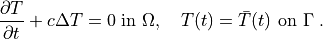
The weak formulation of (1) is: Find $T \in V$ , such that

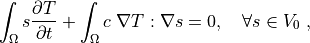
(2)¶ $\int_{\Omega} s \pdiff{T}{t} + \int_{\Omega} c\ \nabla T : \nabla s = 0, \quad \forall s \in V_0 \;,$

where we assume no fluxes over $\partial \Omega \setminus \Gamma$ . In the syntax used in SfePy input files, this can be written as:

dw_dot.i.Omega( s, dT/dt ) + dw_laplace.i.Omega( coef, s, T) = 0

which directly corresponds to the discrete version of (2): Find $\bm{T} \in V_h$ , such that

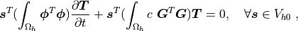
$\bm{s}^T (\int_{\Omega_h} \bm{\phi}^T \bm{\phi}) \pdiff{\bm{T}}{t} + \bm{s}^T (\int_{\Omega_h} c\ \bm{G}^T \bm{G}) \bm{T} = 0, \quad \forall \bm{s} \in V_{h0} \;,$

where $u \approx \bm{\phi} \bm{u}$ , $\nabla u \approx \bm{G} \bm{u}$ for $u \in \{s, T\}$ . The integrals over the discrete domain $\Omega_h$ are approximated by a numerical quadrature, that is named $\verb|i|$ in our case.

Syntax of Terms in Equations ¶

The terms in equations are written in form:

<term_name>.<i>.<r>( <arg1>, <arg2>, ... )

where <i> denotes an integral name (i.e. a name of numerical quadrature to use) and <r> marks a region (domain of the integral). In the following, <virtual> corresponds to a test function, <state> to a unknown function and <parameter> to a known function arguments.

When solving, the individual terms in equations are evaluated in the ‘weak’ mode. The evaluation modes are described in the next section.

Term Evaluation ¶

Terms can be evaluated in two ways:

implicitly by using them in equations;
explicitly using Problem.evaluate(). This way is mostly used in the postprocessing.

Each term supports one or more evaluation modes:

‘weak’ : Assemble (in the finite element sense) either the vector or matrix depending on diff_var argument (the name of variable to differentiate with respect to) of Term.evaluate(). This mode is usually used implicitly when building the linear system corresponding to given equations.
‘eval’ : The evaluation mode integrates the term (= integral) over a region. The result has the same dimension as the quantity being integrated. This mode can be used, for example, to compute some global quantities during postprocessing such as fluxes or total values of extensive quantities (mass, volume, energy, …).
‘el_eval’ : The element evaluation mode results in an array of a quantity integrated over each element of a region.
‘el_avg’ : The element average mode results in an array of a quantity averaged in each element of a region. This is the mode for postprocessing.
‘qp’ : The quadrature points mode results in an array of a quantity interpolated into quadrature points of each element in a region. This mode is used when further point-wise calculations with the result are needed. The same element type and number of quadrature points in each element are assumed.

Not all terms support all the modes - consult the documentation of the individual terms. There are, however, certain naming conventions:

‘dw_*’ terms support ‘weak’ mode
‘dq_*’ terms support ‘qp’ mode
‘d_*’, ‘di_*’ terms support ‘eval’ and ‘el_eval’ modes
‘ev_*’ terms support ‘eval’, ‘el_eval’, ‘el_avg’ and ‘qp’ modes

Note that the naming prefixes are due to history when the mode argument to Problem.evaluate() and Term.evaluate() was not available. Now they are often redundant, but are kept around to indicate the evaluation purpose of each term.

Several examples of using the Problem.evaluate() function are shown below.

Solution Postprocessing ¶

A solution to equations given in a problem description file is given by the variables of the ‘unknown field’ kind, that are set in the solution procedure. By default, those are the only values that are stored into a results file. The solution postprocessing allows computing additional, derived, quantities, based on the primary variables values, as well as any other quantities to be stored in the results.

Let us illustrate this using several typical examples. Let us assume that the postprocessing function is called ‘post_process()’, and is added to options as discussed in Miscellaneous, see ‘post_process_hook’ and ‘post_process_hook_final’. Then:

compute stress and strain given the displacements (variable u):

def post_process(out, problem, variables, extend=False):
    """
    This will be called after the problem is solved.

    Parameters
    ----------
    out : dict
        The output dictionary, where this function will store additional
        data.
    problem : Problem instance
        The current Problem instance.
    variables : Variables instance
        The computed state, containing FE coefficients of all the unknown
        variables.
    extend : bool
        The flag indicating whether to extend the output data to the whole
        domain. It can be ignored if the problem is solved on the whole
        domain already.

    Returns
    -------
    out : dict
        The updated output dictionary.
    """
    from sfepy.base.base import Struct

    # Cauchy strain averaged in elements.
    strain = problem.evaluate('ev_cauchy_strain.i.Omega(u)',
                              mode='el_avg')
    out['cauchy_strain'] = Struct(name='output_data',
                                  mode='cell', data=strain,
                                  dofs=None)
    # Cauchy stress averaged in elements.
    stress = problem.evaluate('ev_cauchy_stress.i.Omega(solid.D, u)',
                              mode='el_avg')
    out['cauchy_stress'] = Struct(name='output_data',
                                  mode='cell', data=stress,
                                  dofs=None)

    return out

The full example is linear_elasticity/linear_elastic_probes.py.

compute diffusion velocity given the pressure:

def post_process(out, pb, state, extend=False):
    from sfepy.base.base import Struct

    dvel = pb.evaluate('ev_diffusion_velocity.i.Omega(m.K, p)',
                       mode='el_avg')
    out['dvel'] = Struct(name='output_data',
                         mode='cell', data=dvel, dofs=None)

    return out

The full example is biot-biot_npbc.

store values of a non-homogeneous material parameter:

def post_process(out, pb, state, extend=False):
    from sfepy.base.base import Struct

    mu = pb.evaluate('ev_integrate_mat.2.Omega(nonlinear.mu, u)',
                     mode='el_avg', copy_materials=False, verbose=False)
    out['mu'] = Struct(name='mu', mode='cell', data=mu, dofs=None)

    return out

The full example is linear_elasticity/material_nonlinearity.py.

compute volume of a region (u is any variable defined in the region Omega):
```
volume = problem.evaluate('ev_volume.2.Omega(u)')
```

Probing ¶

Probing applies interpolation to output the solution along specified paths. There are two ways of probing:

VTK probes: It is the simple way of probing using the ‘post_process_hook’. It generates matplotlib figures with the probing results and previews of the mesh with the probe paths. See Primer or linear_elasticity/its2D_5.py example.
SfePy probes: As mentioned in Miscellaneous, it relies on defining two additional functions, namely the ‘gen_probes’ function, that should create the required probes (see sfepy.discrete.probes), and the ‘probe_hook’ function that performs the actual probing of the results for each of the probes. This function can return the probing results, as well as a handle to a corresponding matplotlib figure. See linear_elasticity/its2D_4.py for additional explanation.

Using sfepy.discrete.probes allows correct probing of fields with the approximation order greater than one, see Interactive Example in Primer or linear_elasticity/its2D_interactive.py for an example of interactive use.

Postprocessing filters ¶

The following postprocessing functions based on the VTK filters are available:

‘get_vtk_surface’: extract mesh surface
‘get_vtk_edges’: extract mesh edges
‘get_vtk_by_group’: extract domain by a material ID
‘tetrahedralize_vtk_mesh’: 3D cells are converted to tetrahedral meshes, 2D cells to triangles

The following code demonstrates the use of the postprocessing filters:

mesh = problem.domain.mesh
mesh_name = mesh.name[mesh.name.rfind(osp.sep) + 1:]

vtkdata = get_vtk_from_mesh(mesh, out, 'postproc_')
matrix = get_vtk_by_group(vtkdata, 1, 1)

matrix_surf = get_vtk_surface(matrix)
matrix_surf_tri = tetrahedralize_vtk_mesh(matrix_surf)
write_vtk_to_file('%s_mat1_surface.vtk' % mesh_name, matrix_surf_tri)

matrix_edges = get_vtk_edges(matrix)
write_vtk_to_file('%s_mat1_edges.vtk' % mesh_name, matrix_edges)

Solvers ¶

This section describes the time-stepping, nonlinear, linear, eigenvalue and optimization solvers available in SfePy. There are many internal and external solvers in the sfepy.solvers package that can be called using a uniform interface.

Time-stepping solvers ¶

All PDEs that can be described in a problem description file are solved internally by a time-stepping solver. This holds even for stationary problems, where the default single-step solver ('ts.stationary') is created automatically. In this way, all problems are treated in a uniform way. The same holds when building a problem interactively, or when writing a script, whenever the Problem.solve() function is used for a problem solution.

The following solvers are available:

ts.adaptive: Implicit time stepping solver with an adaptive time step.
ts.bathe: Solve elastodynamics problems by the Bathe method.
ts.central_difference: Solve elastodynamics problems by the explicit central difference method.
ts.euler: Simple forward euler method
ts.generalized_alpha: Solve elastodynamics problems by the generalized $\alpha$ method.
ts.multistaged: Explicit time stepping solver with multistage solve_step method
ts.newmark: Solve elastodynamics problems by the Newmark method.
ts.runge_kutta_4: Classical 4th order Runge-Kutta method,
ts.simple: Implicit time stepping solver with a fixed time step.
ts.stationary: Solver for stationary problems without time stepping.
ts.tvd_runge_kutta_3: 3rd order Total Variation Diminishing Runge-Kutta method
ts.velocity_verlet: Solve elastodynamics problems by the explicit velocity-Verlet method.

See sfepy.solvers.ts_solvers for available time-stepping solvers and their options.

The following time step controllers are available:

tsc.ed_basic: Adaptive time step I-controller for elastodynamics.
tsc.ed_linear: Adaptive time step controller for elastodynamics and linear problems.
tsc.ed_pid: Adaptive time step PID controller for elastodynamics.
tsc.fixed: Fixed (do-nothing) time step controller.
tsc.time_sequence: Given times sequence time step controller.

See sfepy.solvers.ts_controllers for available time step controllers and their options.

Nonlinear Solvers ¶

Almost every problem, even linear, is solved in SfePy using a nonlinear solver that calls a linear solver in each iteration. This approach unifies treatment of linear and non-linear problems, and simplifies application of Dirichlet (essential) boundary conditions, as the linear system computes not a solution, but a solution increment, i.e., it always has zero boundary conditions.

The following solvers are available:

nls.newton: Solves a nonlinear system $f(x) = 0$ using the Newton method.
nls.oseen: The Oseen solver for Navier-Stokes equations.
nls.petsc: Interface to PETSc SNES (Scalable Nonlinear Equations Solvers).
nls.scipy_broyden_like: Interface to Broyden and Anderson solvers from scipy.optimize.
nls.semismooth_newton: The semi-smooth Newton method.

See sfepy.solvers.nls, sfepy.solvers.oseen and sfepy.solvers.semismooth_newton for all available nonlinear solvers and their options.

Linear Solvers ¶

Choosing a suitable linear solver is key to solving efficiently stationary as well as transient PDEs. SfePy allows using a number of external solvers with a unified interface.

The following solvers are available:

ls.cholesky: Interface to scikit-sparse.cholesky solver.
ls.cm_pb: Conjugate multiple problems.
ls.mumps: Interface to MUMPS solver.
ls.mumps_par: Interface to MUMPS parallel solver.
ls.petsc: PETSc Krylov subspace solver.
ls.pyamg: Interface to PyAMG solvers.
ls.pyamg_krylov: Interface to PyAMG Krylov solvers.
ls.rmm: Special solver for explicit transient elastodynamics.
ls.schur_mumps: Mumps Schur complement solver.
ls.scipy_direct: Direct sparse solver from SciPy.
ls.scipy_iterative: Interface to SciPy iterative solvers.
ls.scipy_superlu: SuperLU - direct sparse solver from SciPy.
ls.scipy_umfpack: UMFPACK - direct sparse solver from SciPy.

See sfepy.solvers.ls for all available linear solvers and their options.

Virtual Linear Solvers with Automatic Selection ¶

A “virtual” solver can be used in case it is not clear which external linear solvers are available. Each “virtual” solver selects the first available solver from a pre-defined list.

The following solvers are available:

ls.auto_direct: The automatically selected linear direct solver.
ls.auto_iterative: The automatically selected linear iterative solver.

See sfepy.solvers.auto_fallback for all available virtual solvers.

Eigenvalue Problem Solvers ¶

The following eigenvalue problem solvers are available:

eig.matlab: Matlab eigenvalue problem solver.
eig.octave: Octave eigenvalue problem solver.
eig.primme: PRIMME eigenvalue problem solver.
eig.scipy: SciPy-based solver for both dense and sparse problems.
eig.scipy_lobpcg: SciPy-based LOBPCG solver for sparse symmetric problems.
eig.sgscipy: SciPy-based solver for dense symmetric problems.
eig.slepc: General SLEPc eigenvalue problem solver.

See sfepy.solvers.eigen for available eigenvalue problem solvers and their options.

Quadratic Eigenvalue Problem Solvers ¶

The following quadratic eigenvalue problem solvers are available:

eig.qevp: Quadratic eigenvalue problem solver based on the problem linearization.

See sfepy.solvers.qeigen for available quadratic eigenvalue problem solvers and their options.

Optimization Solvers ¶

The following optimization solvers are available:

nls.scipy_fmin_like: Interface to SciPy optimization solvers scipy.optimize.fmin_*.
opt.fmin_sd: Steepest descent optimization solver.

See sfepy.solvers.optimize for available optimization solvers and their options.

Solving Problems in Parallel ¶

The PETSc-based nonlinear equations solver 'nls.petsc' and linear system solver 'ls.petsc' can be used for parallel computations, together with the modules in sfepy.parallel package. This feature is very preliminary, and can be used only with the commands for interactive use - problem description files are not supported (yet). The key module is sfepy.parallel.parallel that takes care of the domain and field DOFs distribution among parallel tasks, as well as parallel assembling to PETSc vectors and matrices.

Current Implementation Drawbacks ¶

The partitioning of the domain and fields DOFs is not done in parallel and all tasks need to load the whole mesh and define the global fields - those must fit into memory available to each task.
While all KSP and SNES solver are supported, in principle, most of their options have to be passed using the command-line parameters of PETSc - they are not supported yet in the SfePy solver parameters.
There are no performance statistics yet. The code was tested on a single multi-cpu machine only.
The global solution is gathered to task 0 and saved to disk serially.
The vertices of surface region selector does not work in parallel, because the region definition is applied to a task-local domain.

Examples ¶

The examples demonstrating the use parallel problem solving in SfePy are:

See their help messages for further information.

Isogeometric Analysis ¶

Isogeometric analysis (IGA) is a recently developed computational approach that allows using the NURBS-based domain description from CAD design tools also for approximation purposes similar to the finite element method.

The implementation is SfePy is based on Bezier extraction of NURBS as developed in [1]. This approach allows reusing the existing finite element assembling routines, as still the evaluation of weak forms occurs locally in “elements” and the local contributions are then assembled to the global system.

Current Implementation ¶

The IGA code is still very preliminary and some crucial components are missing. The current implementation is also very slow, as it is in pure Python.

The following already works:

single patch tensor product domain support in 2D and 3D
region selection based on topological Bezier mesh, see below
Dirichlet boundary conditions using projections for non-constant values
evaluation in arbitrary point in the physical domain
both scalar and vector cell terms work
term integration over the whole domain as well as a cell subdomain
simple linearization (output file generation) based on sampling the results with uniform parametric vectors
basic domain generation with sfepy/scripts/gen_iga_patch.py based on igakit

The following is not implemented yet:

tests
theoretical convergence rate verification
facet terms
other boundary conditions
proper (adaptive) linearization for post-processing
support for multiple NURBS patches

Domain Description ¶

The domain description is in custom HDF5-based files with .iga extension. Such a file contains:

NURBS patch data (knots, degrees, control points and weights). Those can either be generated using igakit, created manually or imported from other tools.
Bezier extraction operators and corresponding DOF connectivity (computed by SfePy).
Bezier mesh control points, weights and connectivity (computed by SfePy).

The Bezier mesh is used to create a topological Bezier mesh - a subset of the Bezier mesh containing the Bezier element corner vertices only. Those vertices are interpolatory (are on the exact geometry) and so can be used for region selections.

Region Selection ¶

The domain description files contain vertex sets for regions corresponding to the patch sides, named 'xiIJ', where I is the parametric axis (0, 1, or 2) and J is 0 or 1 for the beginning and end of the axis knot span. Other regions can be defined in the usual way, using the topological Bezier mesh entities.

Examples ¶

The examples demonstrating the use of IGA in SfePy are:

Their problem description files are almost the same as their FEM equivalents, with the following differences:

There is filename_domain instead of filename_mesh.
Fields are defined as follows:
```
fields = {
    't1' : ('real', 1, 'Omega', None, 'H1', 'iga'),
    't2' : ('real', 1, 'Omega', 'iga', 'H1', 'iga'),
    't3' : ('real', 1, 'Omega', 'iga+%d', 'H1', 'iga'),
}
```
The approximation order in the first definition is None as it is given by the NURBS degrees in the domain description. The second definition is equivalent to the first one. The third definition, where %d should be a non-negative integer, illustrates how to increase the field’s NURBS degrees (while keeping the continuity) w.r.t. the domain NURBS description. It is applied in the navier_stokes/navier_stokes2d_iga.py example to the velocity field.