Tutorial
Basic SfePy Usage
SfePy package can be used in two basic ways as a:
Black-box Partial Differential Equation (PDE) solver,
Python package to build custom applications involving solving PDEs by the Finite Element Method (FEM).
This tutorial focuses on the first way and introduces the basic concepts and nomenclature used in the following parts of the documentation. Check also the Primer which focuses on a particular problem in detail.
Users not familiar with the finite element method should start with the Notes on solving PDEs by the Finite Element Method.
Invoking SfePy from the Command Line
This section introduces the basics of running SfePy from the command line, assuming it was properly installed, see Installation.
The command sfepy-run is the most basic starting point in SfePy. It can be used to run declarative problem description files (see below) as follows:
sfepy-run <problem_description_file>
Using SfePy Interactively
All functions of SfePy package can be also used interactively (see Interactive Example: Linear Elasticity for instance).
We recommend to use the IPython interactive shell for the best fluent user experience.
Basic Notions
The simplest way of using SfePy is to solve a system of PDEs defined in a problem description file, also referred to as input file. In such a file, the problem is described using several keywords that allow one to define the equations, variables, finite element approximations, solvers and solution domain and subdomains (see sec-problem-description-file for a full list of those keywords).
The syntax of the problem description file is very simple yet powerful, as the file itself is just a regular Python module that can be normally imported – no special parsing is necessary. The keywords mentioned above are regular Python variables (usually of the dict type) with special names.
Below we show:
how to solve a problem given by a problem description file, and
explain the elements of the file on several examples.
But let us begin with a slight detour…
Sneak Peek: What is Going on Under the Hood
A command (usually sfepy-run as in this tutorial) or a script reads in an input file.
Following the contents of the input file, a Problem instance is created – this is the input file coming to life. Let us call the instance problem.
The Problem instance sets up its domain, regions (various sub-domains), fields (the FE approximations), the equations and the solvers. The equations determine the materials and variables in use – only those are fully instantiated, so the input file can safely contain definitions of items that are not used actually.
The solution is then obtained by calling problem.solve() function, which in turn calls a top-level time-stepping solver. In each step, problem.time_update() is called to setup boundary conditions, material parameters and other potentially time-dependent data. The problem.save_state() is called at the end of each time step to save the results. This holds also for stationary problems with a single “time step”.
So that is it – using the code a black-box PDE solver shields the user from having to create the Problem instance by hand. But note that this is possible, and often necessary when the flexibility of the default solvers is not enough. At the end of the tutorial an example demonstrating the interactive creation of the Problem instance is shown, see Interactive Example: Linear Elasticity.
Now let us continue with running a simulation.
Running a Simulation
The following commands should be run in the top-level directory of the SfePy source tree after compiling the C extension files. See Installation for full installation instructions.
Download
sfepy/examples/diffusion/poisson_short_syntax.py. It represents our sample SfePy sec-problem-description-file, which defines the problem to be solved in terms SfePy can understand.Use the downloaded file in place of <problem_description_file.py> and run sfepy-run as described above. The successful execution of the command creates output file
cylinder.vtkin the SfePy top-level directory.
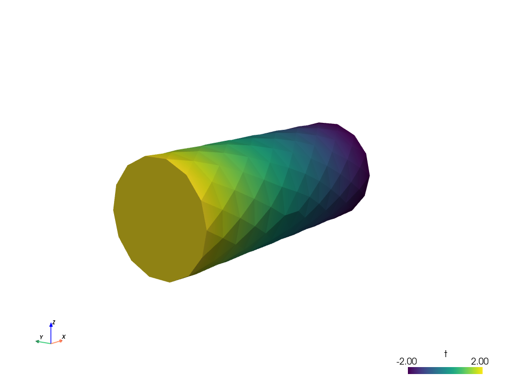
Postprocessing the Results
The sfepy-view command can be used for quick postprocessing and visualization of the SfePy output files. It requires pyvista installed on your system.
As a simple example, try:
sfepy-view cylinder.vtk
The following interactive 3D window should display:
You can manipulate displayed image using:
the left mouse button by itself orbits the 3D view,
holding shift and the left mouse button pans the view,
holding control and the left mouse button rotates about the screen normal axis,
the right mouse button controls the zoom.
Example Problem Description File
Here we discuss the contents of the
sfepy/examples/diffusion/poisson_short_syntax.py problem description file. For
additional examples, see the problem description files in the
sfepy/examples/ directory of SfePy.
The problem at hand is the following:
(1)
where  is a subset of the domain
  boundary. For simplicity, we set
  , but we still work with
the material constant
, but we still work with
the material constant  even though it has no influence on the
solution in this case. We also assume zero fluxes over
even though it has no influence on the
solution in this case. We also assume zero fluxes over  , i.e.
  there. The
particular boundary conditions used below are
there. The
particular boundary conditions used below are  on the left side
of the cylindrical domain depicted in the previous section and
on the left side
of the cylindrical domain depicted in the previous section and  on the right side.
The first step to do is to write (1) in weak
formulation (5). The  ,
,
 . So only one term in weak form
(5) remains:
. So only one term in weak form
(5) remains:
(2)
Comparing the above integral term with the long table in Term Overview, we can see that SfePy contains this term under name dw_laplace. We are now ready to proceed to the actual problem definition.
Open the sfepy/examples/diffusion/poisson_short_syntax.py file in your favorite text
editor. Note that the file is a regular Python source code.
from sfepy import data_dir

filename_mesh = data_dir + '/meshes/3d/cylinder.mesh'
The filename_mesh variable points to the file containing the mesh for the particular problem. SfePy supports a variety of mesh formats.
materials = {
    'coef': ({'val' : 1.0},),
}
Here we define just a constant coefficient of the Poisson
equation, using the ‘values’ attribute. Other possible attribute is
‘function’ for material coefficients computed/obtained at runtime.
Many finite element problems require the definition of material parameters. These can be handled in SfePy with material variables which associate the material parameters with the corresponding region of the mesh.
regions = {
    'Omega' : 'all', # or 'cells of group 6'
    'Gamma_Left' : ('vertices in (x < 0.00001)', 'facet'),
    'Gamma_Right' : ('vertices in (x > 0.099999)', 'facet'),
}
Regions assign names to various parts of the finite element mesh. The region names can later be referred to, for example when specifying portions of the mesh to apply boundary conditions to. Regions can be specified in a variety of ways, including by element or by node. Here, ‘Omega’ is the elemental domain over which the PDE is solved and ‘Gamma_Left’ and ‘Gamma_Right’ define surfaces upon which the boundary conditions will be applied.
fields = {
    'temperature': ('real', 1, 'Omega', 1)
}
A field is used mainly to define the approximation on a (sub)domain, i.e. to
define the discrete spaces  , where we seek the solution.
The Poisson equation can be used to compute e.g. a temperature distribution, so let us call our field ‘temperature’. On the region ‘Omega’ it will be approximated using linear finite elements.
A field in a given region defines the finite element approximation. Several variables can use the same field, see below.
variables = {
    't': ('unknown field', 'temperature', 0),
    's': ('test field', 'temperature', 't'),
}
One field can be used to generate discrete degrees of freedom (DOFs) of several variables. Here the unknown variable (the temperature) is called ‘t’, it’s associated DOF name is ‘t.0’ – this will be referred to in the Dirichlet boundary section (ebc). The corresponding test variable of the weak formulation is called ‘s’. Notice that the ‘dual’ item of a test variable must specify the unknown it corresponds to.
For each unknown (or state) variable there has to be a test (or virtual) variable defined, as usual in weak formulation of PDEs.
ebcs = {
    't1': ('Gamma_Left', {'t.0' : 2.0}),
    't2', ('Gamma_Right', {'t.0' : -2.0}),
}
Essential (Dirichlet) boundary conditions can be specified as above.
Boundary conditions place restrictions on the finite element formulation and create a unique solution to the problem. Here, we specify that a temperature of +2 is applied to the left surface of the mesh and a temperature of -2 is applied to the right surface.
integrals = {
    'i': 2,
}
Integrals specify which numerical scheme to use. Here we are using a 2nd order quadrature over a 3 dimensional space.
equations = {
    'Temperature' : """dw_laplace.i.Omega( coef.val, s, t ) = 0"""
}
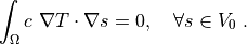
The equation above directly corresponds to the discrete version of
(2), namely: Find  , such that
where  .
.
The equations block is the heart of the SfePy problem description file. Here, we are specifying that the Laplacian of the temperature (in the weak formulation) is 0, where coef.val is a material constant. We are using the ‘i’ integral defined previously, over the domain specified by the region ‘Omega’.
The above syntax is useful for defining custom integrals with user-defined quadrature points and weights, see Integrals. The above uniform integration can be more easily achieved by:
equations = {
    'Temperature' : """dw_laplace.2.Omega( coef.val, s, t ) = 0"""
}
The integration order is specified directly in place of the integral name. The integral definition is superfluous in this case.
solvers = {
    'ls' : ('ls.scipy_direct', {}),
    'newton' : ('nls.newton',
                {'i_max'      : 1,
                 'eps_a'      : 1e-10,
    }),
}
Here, we specify the linear and nonlinear solver kinds and options. See
sfepy.solvers.ls, sfepy.solvers.nls and
sfepy.solvers.ts_solvers for available solvers and their parameters..
Even linear problems are solved by a nonlinear solver (KISS rule) – only one
iteration is needed and the final residual is obtained for free. Note that we
do not need to define a time-stepping solver here - the problem is stationary
and the default 'ts.stationary' solver is created automatically.
options = {
    'nls' : 'newton',
    'ls' : 'ls',
}
The solvers to use are specified in the options block. We can define multiple solvers with different convergence parameters.
That’s it! Now it is possible to proceed as described in Invoking SfePy from the Command Line.
Interactive Example: Linear Elasticity
This example shows how to use SfePy interactively, but also how to make a custom simulation script. We will use IPython interactive shell which allows more flexible and intuitive work (but you can use standard Python shell as well).
We wish to solve the following linear elasticity problem:
(3)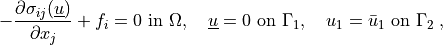
where the stress is defined as  ,
,  ,
,  are the Lamé’s
constants, the strain is
are the Lamé’s
constants, the strain is  and
and  are
volume forces. This can be written in general form as
are
volume forces. This can be written in general form as
 , where in our case
 .
.
In the weak form the equation (3) is
(4)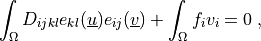
where  is the test function, and both
  ,
belong to a suitable function space.
,
belong to a suitable function space.
Hint: Whenever you create a new object (e.g. a Mesh instance, see below), try to print it using the print statement – it will give you insight about the object internals.
The whole example summarized in a script is available below in Complete Example as a Script.
In the SfePy top-level directory run
ipython
In [1]: import numpy as nm
In [2]: from sfepy.discrete.fem import Mesh, FEDomain, Field
Read a finite element mesh, that defines the domain .
In [3]: mesh = Mesh.from_file('meshes/2d/rectangle_tri.mesh')
Create a domain. The domain allows defining regions or subdomains.
In [4]: domain = FEDomain('domain', mesh)
Define the regions – the whole domain , where the solution
is sought, and  ,
,  , where the boundary
conditions will be applied. As the domain is rectangular, we first get a
bounding box to get correct bounds for selecting the boundary edges.
, where the boundary
conditions will be applied. As the domain is rectangular, we first get a
bounding box to get correct bounds for selecting the boundary edges.
In [5]: min_x, max_x = domain.get_mesh_bounding_box()[:, 0]
In [6]: eps = 1e-8 * (max_x - min_x)
In [7]: omega = domain.create_region('Omega', 'all')
In [8]: gamma1 = domain.create_region('Gamma1',
   ...:                               'vertices in x < %.10f' % (min_x + eps),
   ...:                               'facet')
In [9]: gamma2 = domain.create_region('Gamma2',
   ...:                               'vertices in x > %.10f' % (max_x - eps),
   ...:                               'facet')
Next we define the actual finite element approximation using the
Field class.
In [10]: field = Field.from_args('fu', nm.float64, 'vector', omega,
   ....:                         approx_order=2)
Using the field fu, we can define both the unknown variable  and
the test variable
and
the test variable  .
.
In [11]: from sfepy.discrete import (FieldVariable, Material, Integral, Function,
   ....:                             Equation, Equations, Problem)

In [12]: u = FieldVariable('u', 'unknown', field)
In [13]: v = FieldVariable('v', 'test', field, primary_var_name='u')
Before we can define the terms to build the equation of linear
elasticity, we have to create also the materials, i.e. define the
(constitutive) parameters. The linear elastic material m will be
defined using the two Lamé constants  ,
,  . The volume forces will be defined also as a material as a constant
(column) vector
. The volume forces will be defined also as a material as a constant
(column) vector ![[0.02, 0.01]^T](_images/math/96193b744912167b2566c22f4b43797986e086db.png) .
.
In [14]: from sfepy.mechanics.matcoefs import stiffness_from_lame

In [15]: m = Material('m', D=stiffness_from_lame(dim=2, lam=1.0, mu=1.0))
In [16]: f = Material('f', val=[[0.02], [0.01]])
One more thing needs to be defined – the numerical quadrature that will be used to integrate each term over its domain.
In [17]: integral = Integral('i', order=3)
Now we are ready to define the two terms and build the equations.
In [18]: from sfepy.terms import Term

In [19]: t1 = Term.new('dw_lin_elastic(m.D, v, u)',
   ....:               integral, omega, m=m, v=v, u=u)

In [20]: t2 = Term.new('dw_volume_lvf(f.val, v)',
   ....:               integral, omega, f=f, v=v)
In [21]: eq = Equation('balance', t1 + t2)
In [22]: eqs = Equations([eq])
The equations have to be completed by boundary conditions. Let us clamp
the left edge , and shift the right edge
in the  direction a bit, depending on the
 coordinate.
In [23]: from sfepy.discrete.conditions import Conditions, EssentialBC

In [24]: fix_u = EssentialBC('fix_u', gamma1, {'u.all' : 0.0})
In [25]: def shift_u_fun(ts, coors, bc=None, problem=None, shift=0.0):
   ....:                 val = shift * coors[:,1]**2
   ....:                 return val
In [26]: bc_fun = Function('shift_u_fun', shift_u_fun,
   ....:                   extra_args={'shift' : 0.01})
In [27]: shift_u = EssentialBC('shift_u', gamma2, {'u.0' : bc_fun})
The last thing to define before building the problem are the solvers. Here we just use a sparse direct SciPy solver and the SfePy Newton solver with default parameters. We also wish to store the convergence statistics of the Newton solver. As the problem is linear it should converge in one iteration.
In [28]: from sfepy.base.base import IndexedStruct
In [29]: from sfepy.solvers.ls import ScipyDirect
In [30]: from sfepy.solvers.nls import Newton

In [31]: ls = ScipyDirect({})
In [32]: nls_status = IndexedStruct()
In [33]: nls = Newton({}, lin_solver=ls, status=nls_status)
Now we are ready to create a Problem instance.
In [34]: pb = Problem('elasticity', equations=eqs)
The Problem has several handy methods
for debugging. Let us try saving the regions into a VTK file.
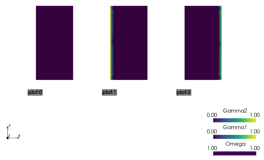
In [35]: pb.save_regions_as_groups('regions')
And view them
In [36]: ! sfepy-view regions.vtk -2 --grid-vector1 "[2, 0, 0]"
You should see this:
Finally, we set the boundary conditions and the top-level solver , solve the
problem, save and view the results. For stationary problems, the top-level
solver needs not to be a time-stepping solver - when a nonlinear solver is set
instead, the default 'ts.stationary' time-stepping solver is created
automatically.
In [39]: pb.set_bcs(ebcs=Conditions([fix_u, shift_u]))
In [40]: pb.set_solver(nls)

In [41]: status = IndexedStruct()
In [42]: variables = pb.solve(status=status)

In [43]: print('Nonlinear solver status:\n', nls_status)
In [44]: print('Stationary solver status:\n', status)

In [45]: pb.save_state('linear_elasticity.vtk', variables)
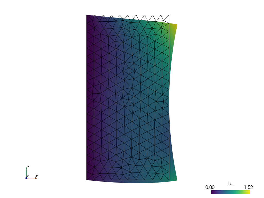
This
sfepy-view linear_elasticity.vtk -2
is used to produce the resulting image:
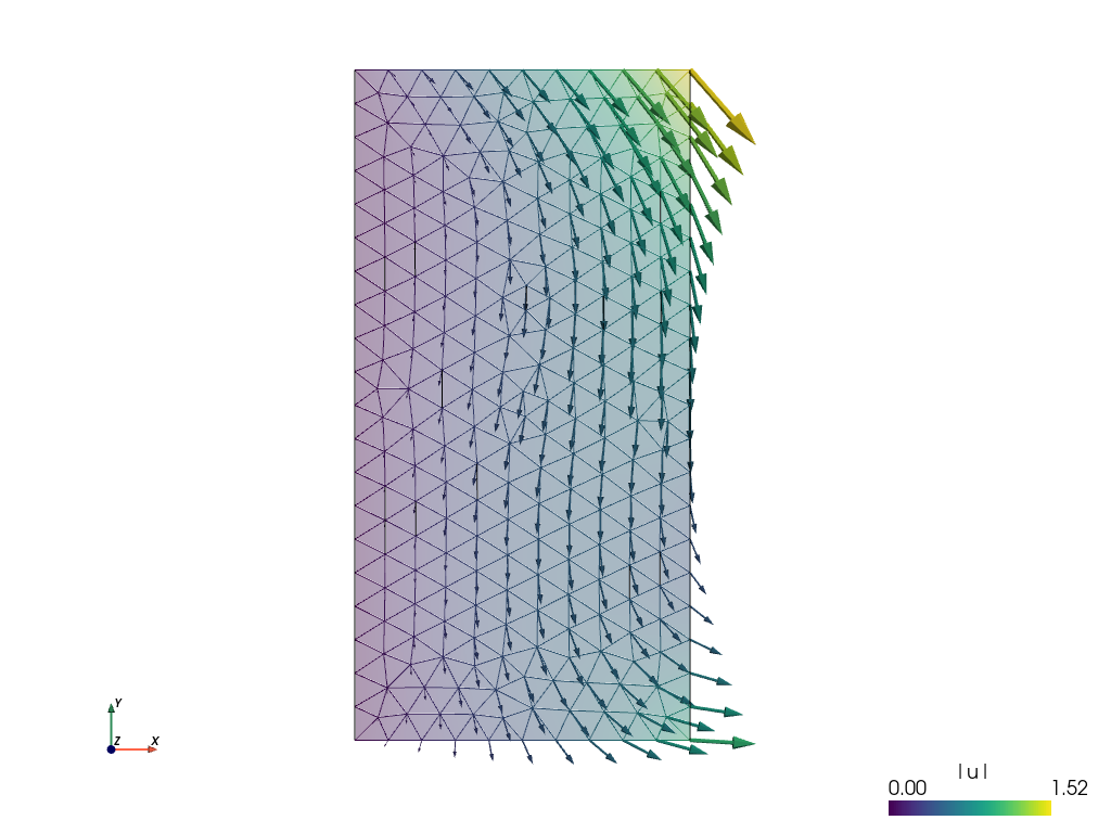
The default view is not very fancy. Let us show the displacements by shifting the mesh. Close the previous window and do
sfepy-view linear_elasticity.vtk -2 -f u:wu:p0 1:vw:p0
And the result is:
Complete Example as a Script
The source code: linear_elastic_interactive.py.
This file should be run from the top-level SfePy source directory so it can find the mesh file correctly. Please note that the provided example script may differ from above tutorial in some minor details.
 1#!/usr/bin/env python
 2"""
 3Linear elasticity example using the imperative API.
 4"""
 5from argparse import ArgumentParser
 6import numpy as nm
 7
 8import sys
 9sys.path.append('.')
10
11from sfepy.base.base import IndexedStruct
12from sfepy.discrete import (FieldVariable, Material, Integral, Function,
13                            Equation, Equations, Problem)
14from sfepy.discrete.fem import Mesh, FEDomain, Field
15from sfepy.terms import Term
16from sfepy.discrete.conditions import Conditions, EssentialBC
17from sfepy.solvers.ls import ScipyDirect
18from sfepy.solvers.nls import Newton
19from sfepy.mechanics.matcoefs import stiffness_from_lame
20
21
22def shift_u_fun(ts, coors, bc=None, problem=None, shift=0.0):
23    """
24    Define a displacement depending on the y coordinate.
25    """
26    val = shift * coors[:,1]**2
27
28    return val
29
30
31def main():
32    from sfepy import data_dir
33
34    parser = ArgumentParser()
35    parser.add_argument('--version', action='version', version='%(prog)s')
36    options = parser.parse_args()
37
38    mesh = Mesh.from_file(data_dir + '/meshes/2d/rectangle_tri.mesh')
39    domain = FEDomain('domain', mesh)
40
41    min_x, max_x = domain.get_mesh_bounding_box()[:,0]
42    eps = 1e-8 * (max_x - min_x)
43    omega = domain.create_region('Omega', 'all')
44    gamma1 = domain.create_region('Gamma1',
45                                  'vertices in x < %.10f' % (min_x + eps),
46                                  'facet')
47    gamma2 = domain.create_region('Gamma2',
48                                  'vertices in x > %.10f' % (max_x - eps),
49                                  'facet')
50
51    field = Field.from_args('fu', nm.float64, 'vector', omega,
52                            approx_order=2)
53
54    u = FieldVariable('u', 'unknown', field)
55    v = FieldVariable('v', 'test', field, primary_var_name='u')
56
57    m = Material('m', D=stiffness_from_lame(dim=2, lam=1.0, mu=1.0))
58    f = Material('f', val=[[0.02], [0.01]])
59
60    integral = Integral('i', order=3)
61
62    t1 = Term.new('dw_lin_elastic(m.D, v, u)',
63                  integral, omega, m=m, v=v, u=u)
64    t2 = Term.new('dw_volume_lvf(f.val, v)', integral, omega, f=f, v=v)
65    eq = Equation('balance', t1 + t2)
66    eqs = Equations([eq])
67
68    fix_u = EssentialBC('fix_u', gamma1, {'u.all' : 0.0})
69
70    bc_fun = Function('shift_u_fun', shift_u_fun,
71                      extra_args={'shift' : 0.01})
72    shift_u = EssentialBC('shift_u', gamma2, {'u.0' : bc_fun})
73
74    ls = ScipyDirect({})
75
76    nls_status = IndexedStruct()
77    nls = Newton({}, lin_solver=ls, status=nls_status)
78
79    pb = Problem('elasticity', equations=eqs)
80    pb.save_regions_as_groups('regions')
81
82    pb.set_bcs(ebcs=Conditions([fix_u, shift_u]))
83
84    pb.set_solver(nls)
85
86    status = IndexedStruct()
87    variables = pb.solve(status=status)
88
89    print('Nonlinear solver status:\n', nls_status)
90    print('Stationary solver status:\n', status)
91
92    pb.save_state('linear_elasticity.vtk', variables)
93
94
95if __name__ == '__main__':
96    main()