linear_elasticity/elastodynamic.py
Description
The linear elastodynamics solution of an iron plate impact problem.
Find  such that:
where

Notes
The used elastodynamics solvers expect that the total vector of DOFs contains
three blocks in this order: the displacements, the velocities, and the
accelerations. This is achieved by defining three unknown variables 'u',
'du', 'ddu' and the corresponding test variables, see the variables
definition. Then the solver can automatically extract the mass, damping (zero
here), and stiffness matrices as diagonal blocks of the global matrix. Note
also the use of the 'dw_zero' (do-nothing) term that prevents the
velocity-related variables to be removed from the equations in the absence of a
damping term. This manual declaration of variables and 'dw_zero' can be
avoided by setting the 'auto_transform_equations' option to True, see
linear_elasticity/seismic_load.py or
multi_physics/piezo_elastodynamic.py.
Usage Examples
Run with the default settings (the Newmark method, 3D problem, results stored
in output/ed/):
sfepy-run sfepy/examples/linear_elasticity/elastodynamic.py
Solve using the Bathe method:
sfepy-run sfepy/examples/linear_elasticity/elastodynamic.py -O "tss_name='tsb'"
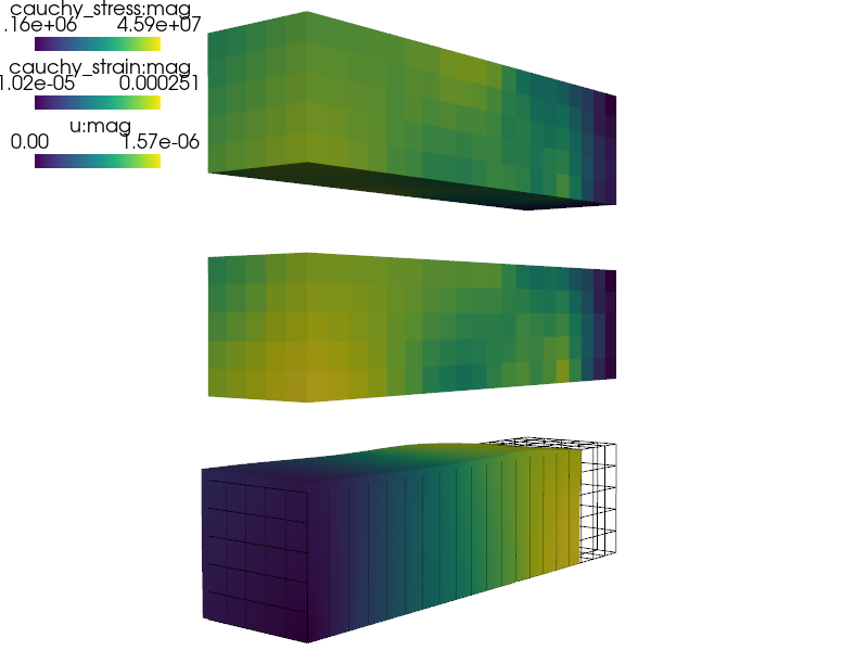
View the resulting displacements on the deforming mesh (1000x magnified), Cauchy strain and stress using:
sfepy-view output/ed/user_block.h5 -f u:wu:f1e3:p0 1:vw:p0 cauchy_strain:p1 cauchy_stress:p2
Solve in 2D using the explicit Velocity-Verlet method with adaptive
time-stepping and save all time steps (see plot_times.py use below):
sfepy-run sfepy/examples/linear_elasticity/elastodynamic.py -d "dims=(5e-3, 5e-3), shape=(61, 61), tss_name='tsvv', tsc_name='tscedb', adaptive=True, save_times='all'"
View the resulting velocities on the deforming mesh (1000x magnified) using:
sfepy-view output/ed/user_block.h5 -2 --grid-vector1=1.2,0,0 -f du:wu:f1e3:p0 1:vw:p0
Plot the adaptive time steps (available at times according to ‘save_times’ option!):
python3 sfepy/scripts/plot_times.py output/ed/user_block.h5 -l
Again, solve in 2D using the explicit Velocity-Verlet method with adaptive time-stepping and save all time steps. Now the used time step control is suitable for linear problems solved by a direct solver: it employs a heuristic that tries to keep the time step size constant for several consecutive steps, reducing so the need for a new matrix factorization. Run:
sfepy-run sfepy/examples/linear_elasticity/elastodynamic.py -d "dims=(5e-3, 5e-3), shape=(61, 61), tss_name='tsvv', tsc_name='tscedl', adaptive=True, save_times='all'"
The resulting velocities and adaptive time steps can again be plotted by the commands shown above.
Use the central difference explicit method with the reciprocal mass matrix algorithm [1] and view the resulting stress waves:
sfepy-run sfepy/examples/linear_elasticity/elastodynamic.py -d "dims=(5e-3, 5e-3), shape=(61, 61), tss_name=tscd, tsc_name=tscedl, adaptive=False, ls_name=lsrmm, mass_beta=0.5, mass_lumping=row_sum, fast_rmm=True, save_times=all"

sfepy-view output/ed/user_block.h5 -2 --grid-vector1=1.2,0,0 -f cauchy_stress:wu:f1e3:p0 1:vw:p0
r"""
The linear elastodynamics solution of an iron plate impact problem.

Find :math:`\ul{u}` such that:

.. math::
    \int_{\Omega} \rho \ul{v} \pddiff{\ul{u}}{t}
    + \int_{\Omega} D_{ijkl}\ e_{ij}(\ul{v}) e_{kl}(\ul{u})
    = 0
    \;, \quad \forall \ul{v} \;,

where

.. math::
    D_{ijkl} = \mu (\delta_{ik} \delta_{jl}+\delta_{il} \delta_{jk}) +
    \lambda \ \delta_{ij} \delta_{kl}
    \;.

Notes
-----

The used elastodynamics solvers expect that the total vector of DOFs contains
three blocks in this order: the displacements, the velocities, and the
accelerations. This is achieved by defining three unknown variables ``'u'``,
``'du'``, ``'ddu'`` and the corresponding test variables, see the `variables`
definition. Then the solver can automatically extract the mass, damping (zero
here), and stiffness matrices as diagonal blocks of the global matrix. Note
also the use of the ``'dw_zero'`` (do-nothing) term that prevents the
velocity-related variables to be removed from the equations in the absence of a
damping term. This manual declaration of variables and ``'dw_zero'`` can be
avoided by setting the ``'auto_transform_equations'`` option to True, see
:ref:`linear_elasticity-seismic_load` or
:ref:`multi_physics-piezo_elastodynamic`.

Usage Examples
--------------

Run with the default settings (the Newmark method, 3D problem, results stored
in ``output/ed/``)::

  sfepy-run sfepy/examples/linear_elasticity/elastodynamic.py

Solve using the Bathe method::

  sfepy-run sfepy/examples/linear_elasticity/elastodynamic.py -O "tss_name='tsb'"

View the resulting displacements on the deforming mesh (1000x magnified),
Cauchy strain and stress using::

  sfepy-view output/ed/user_block.h5 -f u:wu:f1e3:p0 1:vw:p0 cauchy_strain:p1 cauchy_stress:p2

Solve in 2D using the explicit Velocity-Verlet method with adaptive
time-stepping and save all time steps (see ``plot_times.py`` use below)::

  sfepy-run sfepy/examples/linear_elasticity/elastodynamic.py -d "dims=(5e-3, 5e-3), shape=(61, 61), tss_name='tsvv', tsc_name='tscedb', adaptive=True, save_times='all'"

View the resulting velocities on the deforming mesh (1000x magnified) using::

  sfepy-view output/ed/user_block.h5 -2 --grid-vector1=1.2,0,0 -f du:wu:f1e3:p0 1:vw:p0

Plot the adaptive time steps (available at times according to 'save_times'
option!)::

  python3 sfepy/scripts/plot_times.py output/ed/user_block.h5 -l

Again, solve in 2D using the explicit Velocity-Verlet method with adaptive
time-stepping and save all time steps. Now the used time step control is
suitable for linear problems solved by a direct solver: it employs a heuristic
that tries to keep the time step size constant for several consecutive steps,
reducing so the need for a new matrix factorization. Run::

  sfepy-run sfepy/examples/linear_elasticity/elastodynamic.py -d "dims=(5e-3, 5e-3), shape=(61, 61), tss_name='tsvv', tsc_name='tscedl', adaptive=True, save_times='all'"

The resulting velocities and adaptive time steps can again be plotted by the
commands shown above.

Use the central difference explicit method with the reciprocal mass matrix
algorithm [1]_ and view the resulting stress waves::

  sfepy-run sfepy/examples/linear_elasticity/elastodynamic.py -d "dims=(5e-3, 5e-3), shape=(61, 61), tss_name=tscd, tsc_name=tscedl, adaptive=False, ls_name=lsrmm, mass_beta=0.5, mass_lumping=row_sum, fast_rmm=True, save_times=all"

  sfepy-view output/ed/user_block.h5 -2 --grid-vector1=1.2,0,0 -f cauchy_stress:wu:f1e3:p0 1:vw:p0

.. [1] González, J.A., Kolman, R., Cho, S.S., Felippa, C.A., Park, K.C., 2018.
       Inverse mass matrix via the method of localized Lagrange multipliers.
       International Journal for Numerical Methods in Engineering 113, 277–295.
       https://doi.org/10.1002/nme.5613
"""
import numpy as nm

import sfepy.mechanics.matcoefs as mc
from sfepy.discrete.fem.meshio import UserMeshIO
from sfepy.mesh.mesh_generators import gen_block_mesh

def define(
        E=200e9, nu=0.3, rho=7800,
        plane='strain',
        dims=(1e-2, 2.5e-3, 2.5e-3),
        shape=(21, 6, 6),
        v0=1.0,
        ct1=1.5,
        dt=None,
        edt_safety=0.2,
        tss_name='tsn',
        tsc_name='tscedl',
        adaptive=False,
        ls_name='lsd',
        mass_beta=0.0,
        mass_lumping='none',
        fast_rmm=False,
        active_only=False,
        save_times=20,
        output_dir='output/ed',
):
    """
    Parameters
    ----------
    E, nu, rho: material parameters
    plane: plane strain or stress hypothesis
    dims: physical dimensions of the block (L, d, x)
    shape: numbers of mesh vertices along each axis
    v0: initial impact velocity
    ct1: final time in L / "longitudinal wave speed" units
    dt: time step (None means automatic)
    edt_safety: safety factor time step multiplier for explicit schemes,
                if dt is None
    tss_name: time stepping solver name (see "solvers" section)
    tsc_name: time step controller name (see "solvers" section)
    adaptive: use adaptive time step control
    ls_name: linear system solver name (see "solvers" section)
    mass_beta: averaged mass matrix parameter 0 <= beta <= 1
    mass_lumping: mass matrix lumping ('row_sum', 'hrz' or 'none')
    fast_rmm: use zero inertia term with lsrmm
    save_times: number of solutions to save
    output_dir: output directory
    """
    dim = len(dims)

    lam, mu = mc.lame_from_youngpoisson(E, nu, plane=plane)
    # Longitudinal and shear wave propagation speeds.
    cl = nm.sqrt((lam + 2.0 * mu) / rho)
    cs = nm.sqrt(mu / rho)

    # Element size.
    L, d = dims[:2]
    H = L / (nm.max(shape) - 1)

    # Time-stepping parameters.
    if dt is None:
        # For implicit schemes, dt based on the Courant number C0 = dt * cl / H
        # equal to 1.
        dt = H / cl # C0 = 1
        if tss_name in ('tsvv', 'tscd'):
            # For explicit schemes, use a safety margin.
            dt *= edt_safety

    t1 = ct1 * L / cl

    def mesh_hook(mesh, mode):
        """
        Generate the block mesh.
        """
        if mode == 'read':
            mesh = gen_block_mesh(dims, shape, 0.5 * nm.array(dims),
                                  name='user_block', verbose=False)
            return mesh

        elif mode == 'write':
            pass

    def post_process(out, problem, state, extend=False):
        """
        Calculate and output strain and stress for given displacements.
        """
        from sfepy.base.base import Struct

        ev = problem.evaluate
        strain = ev('ev_cauchy_strain.i.Omega(u)', mode='el_avg', verbose=False)
        stress = ev('ev_cauchy_stress.i.Omega(solid.D, u)', mode='el_avg',
                    copy_materials=False, verbose=False)

        out['cauchy_strain'] = Struct(name='output_data', mode='cell',
                                      data=strain)
        out['cauchy_stress'] = Struct(name='output_data', mode='cell',
                                      data=stress)

        return out

    filename_mesh = UserMeshIO(mesh_hook)

    regions = {
        'Omega' : 'all',
        'Impact' : ('vertices in (x < 1e-12)', 'facet'),
    }
    if dim == 3:
        regions.update({
            'Symmetry-y' : ('vertices in (y < 1e-12)', 'facet'),
            'Symmetry-z' : ('vertices in (z < 1e-12)', 'facet'),
        })

    # Iron.
    materials = {
        'solid' : ({
            'D': mc.stiffness_from_youngpoisson(dim=dim, young=E, poisson=nu,
                                                plane=plane),
            'rho': rho,
            '.lumping' : mass_lumping,
            '.beta' : mass_beta,
        },),
    }

    fields = {
        'displacement': ('real', 'vector', 'Omega', 1),
    }

    integrals = {
        'i' : 2,
    }

    # Notes:
    # 1. The order of the variables in the solution vector is specified here
    #    (3rd tuple member), since that specific order is expected by the
    #    elastodynamic time-stepping solvers.
    # 2. For the same reason, we won't explicitly define below the equations
    #    du = du/dt and ddu = ddu/dt - these are implicitly defined by
    #    the time-stepping solver. see the `step()` method of the solvers.
    variables = {
        'u' : ('unknown field', 'displacement', 0),
        'du' : ('unknown field', 'displacement', 1),
        'ddu' : ('unknown field', 'displacement', 2),
        'v' : ('test field', 'displacement', 'u'),
        'dv' : ('test field', 'displacement', 'du'),
        'ddv' : ('test field', 'displacement', 'ddu'),
    }
    # The mapping of variables for the elastodynamics solvers - keys are given,
    # values correspond to the names of the actual variables.
    var_names = {'u' : 'u', 'du' : 'du', 'ddu' : 'ddu'}

    ebcs = {
        'Impact' : ('Impact', {'u.0' : 0.0, 'du.0' : 0.0, 'ddu.0' : 0.0}),
    }
    if dim == 3:
        ebcs.update({
            'Symmtery-y' : ('Symmetry-y',
                            {'u.1' : 0.0, 'du.1' : 0.0, 'ddu.1' : 0.0}),
            'Symmetry-z' : ('Symmetry-z',
                            {'u.2' : 0.0, 'du.2' : 0.0, 'ddu.2' : 0.0}),
        })

    def get_ic(coor, ic, mode='u'):
        val = nm.zeros_like(coor)
        if mode == 'u':
            val[:, 0] = 0.0

        elif mode == 'du':
            val[:, 0] = -1.0

        return val

    functions = {
        'get_ic_u' : (get_ic,),
        'get_ic_du' : (lambda coor, ic: get_ic(coor, None, mode='du'),),
    }

    ics = {
        'ic' : ('Omega', {'u.all' : 'get_ic_u', 'du.all' : 'get_ic_du'}),
    }

    if (ls_name == 'lsrmm') and fast_rmm:
        # Speed up residual calculation, as M is not used with lsrmm.
        term = 'dw_zero.i.Omega(ddv, ddu)'

    else:
        term = 'de_mass.i.Omega(solid.rho, solid.lumping, solid.beta, ddv, ddu)'

    equations = {
        'balance_of_forces' :
        term + """
         + dw_zero.i.Omega(dv, du)
         + dw_lin_elastic.i.Omega(solid.D, v, u) = 0""",
    }

    solvers = {
        'lsd' : ('ls.auto_direct', {
            # Reuse the factorized linear system from the first time step.
            'use_presolve' : True,
            # Speed up the above by omitting the matrix digest check used
            # normally for verification that the current matrix corresponds to
            # the factorized matrix stored in the solver instance. Use with
            # care!
            'use_mtx_digest' : False,
        }),
        'lsi' : ('ls.petsc', {
            'method' : 'cg',
            'precond' : 'icc',
            'i_max' : 150,
            'eps_a' : 1e-32,
            'eps_r' : 1e-8,
            'verbose' : 2,
        }),
        'lsrmm' : ('ls.rmm', {
            'rmm_term' : """de_mass.i.Omega(solid.rho, solid.lumping,
                                            solid.beta, ddv, ddu)""",
            'debug' : False,
        }),
        'newton' : ('nls.newton', {
            'i_max'      : 1,
            'eps_a'      : 1e-6,
            'eps_r'      : 1e-6,
        }),
        'tsvv' : ('ts.velocity_verlet', {
            # Explicit method.
            't0' : 0.0,
            't1' : t1,
            'dt' : dt,
            'n_step' : None,

            'is_linear'  : True,

            'var_names' : var_names,
            'verbose' : 1,
        }),
        'tscd' : ('ts.central_difference', {
            # Explicit method. Supports ls.rmm.
            't0' : 0.0,
            't1' : t1,
            'dt' : dt,
            'n_step' : None,

            'is_linear'  : True,

            'var_names' : var_names,
            'verbose' : 1,
        }),
        'tsn' : ('ts.newmark', {
            't0' : 0.0,
            't1' : t1,
            'dt' : dt,
            'n_step' : None,

            'is_linear'  : True,

            'beta' : 0.25,
            'gamma' : 0.5,

            'var_names' : var_names,
            'verbose' : 1,
        }),
        'tsga' : ('ts.generalized_alpha', {
            't0' : 0.0,
            't1' : t1,
            'dt' : dt,
            'n_step' : None,

            'is_linear'  : True,

            'rho_inf' : 0.5,
            'alpha_m' : None,
            'alpha_f' : None,
            'beta' : None,
            'gamma' : None,

            'var_names' : var_names,
            'verbose' : 1,
        }),
        'tsb' : ('ts.bathe', {
            't0' : 0.0,
            't1' : t1,
            'dt' : dt,
            'n_step' : None,

            'is_linear'  : True,

            'var_names' : var_names,
            'verbose' : 1,
        }),
        'tscedb' : ('tsc.ed_basic', {
            'eps_r' : (1e-4, 1e-1),
            'eps_a' : (1e-8, 5e-2),
            'fmin' : 0.3,
            'fmax' : 2.5,
            'fsafety' : 0.85,
        }),
        'tscedl' : ('tsc.ed_linear', {
            'eps_r' : (1e-4, 1e-1),
            'eps_a' : (1e-8, 5e-2),
            'fmin' : 0.3,
            'fmax' : 2.5,
            'fsafety' : 0.85,
            'red_factor' : 0.9,
            'inc_wait' : 10,
            'min_inc_factor' : 1.5,
        }),
    }

    options = {
        'ts' : tss_name,
        'tsc' : tsc_name if adaptive else None,
        'nls' : 'newton',
        'ls' : ls_name,

        'save_times' : save_times,

        'active_only' : active_only,
        'auto_transform_equations' : False,

        'output_format' : 'h5',
        'output_dir' : output_dir,
        'post_process_hook' : 'post_process',
    }

    return locals()