multi_physics/piezo_elastodynamic.py
Description
The linear elastodynamics of a piezoelectric body loaded by a given base motion.
The generated voltage between the bottom and top surface electrodes is recorded and plotted. The scalar potential on the top surface electrode is modeled using a constant L^2 field. The Nitsche’s method is used to weakly apply the (unknown) potential Dirichlet boundary condition on the top surface.
Find the displacements  , the potential
  and the
constant potential on the top electrode
and the
constant potential on the top electrode  such that:
where  is the matrix of elastic properties under constant
electric field intensity,
is the matrix of elastic properties under constant
electric field intensity,  the piezoelectric modulus,
 the permittivity under constant deformation,
  a
penalty parameter and
a
penalty parameter and  the external circuit resistance (e.g. of an
oscilloscope used to measure the voltage between the electrodes).
the external circuit resistance (e.g. of an
oscilloscope used to measure the voltage between the electrodes).
Usage Examples
Run with the default settings, results stored in output/piezo-ed/:
sfepy-run sfepy/examples/multi_physics/piezo_elastodynamic.py
The define() arguments, see below, can be set using the -d option:
sfepy-run sfepy/examples/multi_physics/piezo_elastodynamic.py -d "order=2, ct1=2.5"
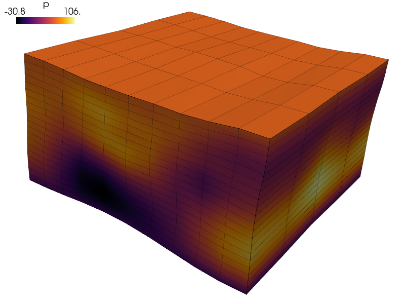
View the resulting potential  on a deformed mesh (2000x magnified):
sfepy-view output/piezo-ed/user_block.h5 -f p:wu:f2000:p0 1:vw:wu:f2000:p0 --color-map=inferno
r"""
The linear elastodynamics of a piezoelectric body loaded by a given base
motion.
The generated voltage between the bottom and top surface electrodes is recorded
and plotted. The scalar potential on the top surface electrode is modeled using
a constant L^2 field. The Nitsche's method is used to weakly apply the
(unknown) potential Dirichlet boundary condition on the top surface.
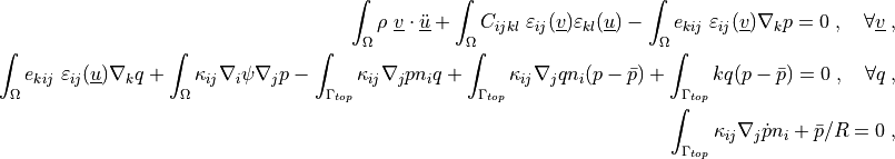
Find the displacements :math:`\ul{u}(t)`, the potential :math:`p(t)` and the
constant potential on the top electrode :math:`\bar p(t)` such that:
.. math::
\int_\Omega \rho\ \ul{v} \cdot \ul{\ddot u}
+ \int_\Omega C_{ijkl}\ \veps_{ij}(\ul{v}) \veps_{kl}(\ul{u})
- \int_\Omega e_{kij}\ \veps_{ij}(\ul{v}) \nabla_k p
= 0
\;, \quad \forall \ul{v} \;,
\int_\Omega e_{kij}\ \veps_{ij}(\ul{u}) \nabla_k q
+ \int_\Omega \kappa_{ij} \nabla_i \psi \nabla_j p
- \int_{\Gamma_{top}} \kappa_{ij} \nabla_j p n_i q
+ \int_{\Gamma_{top}} \kappa_{ij} \nabla_j q n_i (p - \bar p)
+ \int_{\Gamma_{top}} k q (p - \bar p)
= 0
\;, \quad \forall q \;,
\int_{\Gamma_{top}} \kappa_{ij} \nabla_j \dot{p} n_i + \bar p / R = 0 \;,
where :math:`C_{ijkl}` is the matrix of elastic properties under constant
electric field intensity, :math:`e_{kij}` the piezoelectric modulus,
:math:`\kappa_{ij}` the permittivity under constant deformation, :math:`k` a
penalty parameter and :math:`R` the external circuit resistance (e.g. of an
oscilloscope used to measure the voltage between the electrodes).
Usage Examples
--------------
Run with the default settings, results stored in ``output/piezo-ed/``::
sfepy-run sfepy/examples/multi_physics/piezo_elastodynamic.py
The :func:`define()` arguments, see below, can be set using the ``-d`` option::
sfepy-run sfepy/examples/multi_physics/piezo_elastodynamic.py -d "order=2, ct1=2.5"
View the resulting potential :math:`p` on a deformed mesh (2000x magnified)::
sfepy-view output/piezo-ed/user_block.h5 -f p:wu:f2000:p0 1:vw:wu:f2000:p0 --color-map=inferno
"""
from functools import partial
import numpy as nm
from sfepy.base.base import output
from sfepy.discrete.fem.meshio import UserMeshIO
from sfepy.mesh.mesh_generators import gen_block_mesh
from sfepy.homogenization.utils import define_box_regions
def post_process(out, problem, state, extend=False, pcs=None):
"""
Calculate and output strain, stress and electric field vector for the given
displacements and potential.
"""
from sfepy.base.base import Struct
ev = problem.evaluate
strain = ev('ev_cauchy_strain.i.Omega(u)', mode='el_avg', verbose=False)
stress = ev('ev_cauchy_stress.i.Omega(m.C, u)', mode='el_avg',
copy_materials=False, verbose=False)
E = ev('ev_grad.i.Omega(p)', mode='el_avg', verbose=False)
out['cauchy_strain'] = Struct(name='output_data', mode='cell',
data=strain)
out['cauchy_stress'] = Struct(name='output_data', mode='cell',
data=stress)
out['E'] = Struct(name='output_data', mode='cell', data=E)
top = problem.domain.regions['Top']
p_top = state['p'].get_state_in_region(top)
# = state['pc'](), but we want to test .get_state_in_region()
pc_top = state['pc'].get_state_in_region(top)
output('pc:', pc_top)
output('|p - pc|_top:', nm.linalg.norm(p_top - pc_top))
if pcs is not None:
pcs.append(pc_top[0, 0])
return out
def plot_voltage(problem, state, pcs=None):
import os.path as op
import matplotlib.pyplot as plt
ts = problem.get_timestepper()
fig, ax = plt.subplots()
ax.plot(ts.times, pcs)
ax.set_xlabel('$t$ [s]')
ax.set_ylabel(r'$\bar p$ [V]')
fig.tight_layout()
fig.savefig(op.join(problem.output_dir, 'voltage.pdf'))
def define(
dims=(1e-2, 1e-2, 5e-3),
shape=(5, 11, 21),
order=1,
amplitude=0.0000001,
ct1=1.5,
dt=None,
tss_name='tsn',
tsc_name='tscedl',
adaptive=False,
ls_name='lsd',
active_only=False,
save_times='all',
output_dir='output/piezo-ed',
):
"""
Parameters
----------
dims: physical dimensions of the block mesh
shape: numbers of mesh vertices along each axis
order: the FE approximation order
amplitude: the seismic load amplitude
ct1: final time in min(dims) / "longitudinal wave speed" units
dt: time step (None means automatic)
tss_name: time stepping solver name (see "solvers" section)
tsc_name: time step controller name (see "solvers" section)
adaptive: use adaptive time step control
ls_name: linear system solver name (see "solvers" section)
save_times: number of solutions to save
output_dir: output directory
"""
dim = len(dims)
assert dim == 3
# A PZT 5-H material, Voigt notation, strain - electric displacement form.
epsT = nm.array([[1700., 0, 0],
[0, 1700., 0],
[0, 0, 1450.0]])
dv = 1e-12 * nm.array([[0, 0, 0, 0, 741., 0],
[0, 0, 0, 741, 0, 0],
[-274., -274., 593., 0, 0, 0]]) # C / N = m / V
# Convert to stress - electric displacement form.
CEv = nm.array([[1.27e+011, 8.02e+010, 8.47e+010, 0, 0, 0],
[8.02e+010, 1.27e+011, 8.47e+010, 0, 0, 0],
[8.47e+010, 8.47e+010, 1.17e+011, 0, 0, 0],
[0, 0, 0, 2.34e+010, 0, 0],
[0, 0, 0, 0, 2.30e+010, 0],
[0, 0, 0, 0, 0, 2.35e+010]])
ev = dv @ CEv
epsS = epsT - dv @ ev.T
# SfePy: 11 22 33 12 13 23
# Voigt: 11 22 33 23 13 12
ii = [0, 1, 2, 5, 4, 3]
ix, iy = nm.meshgrid(ii, ii, sparse=True)
CE = CEv[ix, iy]
e = ev[:, ii]
eps0 = 8.8541878128e-12
kappa = epsS * eps0
# Longitudinal and shear wave propagation speeds.
mu = CE[-1, -1]
lam = CE[0, 0] - 2 * mu
rho = 7800
cl = nm.sqrt((lam + 2.0 * mu) / rho)
cs = nm.sqrt(mu / rho)
# Element size.
L = nm.min(dims)
H = L / (nm.max(shape) - 1)
# Time-stepping parameters.
if dt is None:
# For implicit schemes, dt based on the Courant number C0 = dt * cl / H
# equal to 1.
dt = H / cl # C0 = 1
t1 = ct1 * L / cl
# Time history record of pc.
pcs = []
_post_process = partial(post_process, pcs=pcs)
_plot_voltage = partial(plot_voltage, pcs=pcs)
def mesh_hook(mesh, mode):
"""
Generate the block mesh.
"""
if mode == 'read':
mesh = gen_block_mesh(dims, shape, 0.5 * nm.array(dims),
name='user_block', verbose=False)
return mesh
elif mode == 'write':
pass
filename_mesh = UserMeshIO(mesh_hook)
bbox = [[0] * dim, dims]
regions = define_box_regions(dim, bbox[0], bbox[1], 1e-5)
regions.update({
'Omega' : 'all',
})
materials = {
'inclusion' : (None, 'get_inclusion_pars')
}
fields = {
'displacement' : ('real', 'vector', 'Omega', order),
'potential' : ('real', 'scalar', 'Omega', order),
'constant' : ('real', 'scalar', 'Top', 0, 'L2', 'constant'),
}
variables = {
'u' : ('unknown field', 'displacement', 0),
'v' : ('test field', 'displacement', 'u'),
'p' : ('unknown field', 'potential', 1, 1),
'q' : ('test field', 'potential', 'p'),
'pc' : ('unknown field', 'constant', 2, 1),
'qc' : ('test field', 'constant', 'pc'),
}
materials = {
'm' : ({
'C': CE,
'e' : e,
'kappa' : kappa,
'rho': rho,
'penalty': 1,
'iR' : 1.0 / (15e6 * dims[0] * dims[1]), # 1 / (R * top_area).
},),
}
integrals = {
'i' : 2 * order,
}
def get_ebcs(ts, coors, mode='u'):
y = coors[:, 1]
k = 2 * nm.pi / dims[1]
shift = nm.pi / 3
omega = cl * k
time = ts.time
if mode == 'u':
val = (amplitude * nm.sin(time * omega) * nm.sin(k * y + shift))
elif mode == 'du':
val = (amplitude * omega * nm.cos(time * omega)
* nm.sin(k * y + shift))
elif mode == 'ddu':
val = (-amplitude * omega**2 * nm.sin(time * omega)
* nm.sin(k * y + shift))
return val
functions = {
'get_u' : (lambda ts, coor, **kwargs: get_ebcs(ts, coor),),
'get_du' : (lambda ts, coor, **kwargs: get_ebcs(ts, coor, mode='du'),),
'get_ddu' : (lambda ts, coor, **kwargs: get_ebcs(ts, coor, mode='ddu'),),
}
ebcs = {
'Seismic' : ('Bottom', {'u.2' : 'get_u', 'du.2' : 'get_du',
'ddu.2' : 'get_ddu'}),
'Pot0' : ('Bottom', {'p.all' : 0.0}),
}
ics = {
'ic' : ('Omega', {'u.all' : 0.0, 'du.all' : 0.0, 'p.0' : 0.0}),
}
equations = {
'1' : """dw_dot.i.Omega(m.rho, v, ddu)
+ dw_lin_elastic.i.Omega(m.C, v, u)
- dw_piezo_coupling.i.Omega(m.e, v, p)
= 0""",
'2' : """dw_piezo_coupling.i.Omega(m.e, u, q)
+ dw_diffusion.i.Omega(m.kappa, q, p)
- de_surface_flux.i.Top(m.kappa, q, p)
+ de_surface_flux.i.Top(m.kappa, p, q)
- de_surface_flux.i.Top(m.kappa, pc, q)
+ dw_dot.i.Top(m.penalty, q, p)
- dw_dot.i.Top(m.penalty, q, pc)
= 0""",
'3' : """de_surface_flux.i.Top(m.kappa, qc, dp/dt)
+ 0.5 * dw_dot.i.Top(m.iR, qc, pc)
+ 0.5 * dw_dot.i.Top(m.iR, qc, pc[-1])
= 0""",
}
solvers = {
'lsd' : ('ls.auto_direct', {
# Reuse the factorized linear system from the first time step.
'use_presolve' : True,
# Speed up the above by omitting the matrix digest check used
# normally for verification that the current matrix corresponds to
# the factorized matrix stored in the solver instance. Use with
# care!
'use_mtx_digest' : False,
# Increase when getting MUMPS error -9.
'memory_relaxation' : 20,
}),
'newton' : ('nls.newton', {
'i_max' : 1,
'eps_a' : 1e-6,
'eps_r' : 1e-6,
'ls_on' : 1e100,
}),
'tsn' : ('ts.newmark', {
't0' : 0.0,
't1' : t1,
'dt' : dt,
'n_step' : None,
'is_linear' : True,
# Without this the adaptive time-stepping cannot work.
'has_time_derivatives' : adaptive,
'beta' : 0.25,
'gamma' : 0.5,
'verbose' : 1,
}),
'tscedl' : ('tsc.ed_linear', {
'eps_r' : (1e-4, 1e-2),
'eps_a' : (1e-8, 1e-3),
'fmin' : 0.3,
'fmax' : 2.5,
'fsafety' : 0.85,
'red_factor' : 0.9,
'inc_wait' : 10,
'min_inc_factor' : 1.5,
}),
}
options = {
'ts' : tss_name,
'tsc' : tsc_name if adaptive else None,
'nls' : 'newton',
'ls' : ls_name,
'save_times' : save_times,
'active_only' : active_only,
'auto_transform_equations' : True,
'output_format' : 'h5',
'output_dir' : output_dir,
'post_process_hook' : _post_process,
'post_process_hook_final' : _plot_voltage,
}
return locals()