large_deformation/perfusion_tl.py

Description

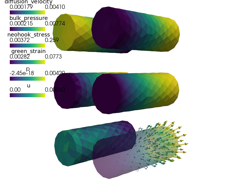
Porous nearly incompressible hyperelastic material with fluid perfusion.

Large deformation is described using the total Lagrangian formulation. Models of this kind can be used in biomechanics to model biological tissues, e.g. muscles.

Find such that:

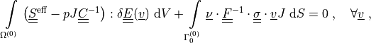
(equilibrium equation with boundary tractions)

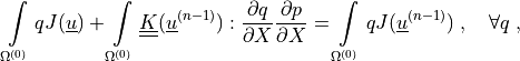
(mass balance equation (perfusion))

where

	deformation gradient
	right Cauchy-Green deformation tensor
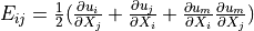
	Green strain tensor
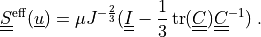
	effective second Piola-Kirchhoff stress tensor

The effective (neo-Hookean) stress is given by:

The linearized deformation-dependent permeability is defined as , where relates to the previous time step and expresses the dependence on volume compression/expansion.

source code

# -*- coding: utf-8 -*-
r"""
Porous nearly incompressible hyperelastic material with fluid perfusion.

Large deformation is described using the total Lagrangian formulation.
Models of this kind can be used in biomechanics to model biological
tissues, e.g. muscles.

Find :math:`\ul{u}` such that:

(equilibrium equation with boundary tractions)

.. math::
    \intl{\Omega\suz}{} \left( \ull{S}\eff - p J \ull{C}^{-1}
    \right) : \delta \ull{E}(\ul{v}) \difd{V}
    + \intl{\Gamma_0\suz}{} \ul{\nu} \cdot \ull{F}^{-1} \cdot \ull{\sigma}
    \cdot  \ul{v} J \difd{S}
    = 0
    \;, \quad \forall \ul{v} \;,

(mass balance equation (perfusion))

.. math::
    \intl{\Omega\suz}{} q J(\ul{u})
    + \intl{\Omega\suz}{} \ull{K}(\ul{u}\sunm) : \pdiff{q}{X} \pdiff{p}{X}
    = \intl{\Omega\suz}{} q J(\ul{u}\sunm)
    \;, \quad \forall q \;,


where

.. list-table::
   :widths: 20 80

   * - :math:`\ull{F}`
     - deformation gradient :math:`F_{ij} = \pdiff{x_i}{X_j}`
   * - :math:`J`
     - :math:`\det(F)`
   * - :math:`\ull{C}`
     -  right Cauchy-Green deformation tensor :math:`C = F^T F`
   * - :math:`\ull{E}(\ul{u})`
     - Green strain tensor :math:`E_{ij} = \frac{1}{2}(\pdiff{u_i}{X_j} +
       \pdiff{u_j}{X_i} + \pdiff{u_m}{X_i}\pdiff{u_m}{X_j})`
   * - :math:`\ull{S}\eff(\ul{u})`
     - effective second Piola-Kirchhoff stress tensor

The effective (neo-Hookean) stress :math:`\ull{S}\eff(\ul{u})` is given
by:

.. math::
    \ull{S}\eff(\ul{u}) = \mu J^{-\frac{2}{3}}(\ull{I}
    - \frac{1}{3}\tr(\ull{C}) \ull{C}^{-1})
    \;.

The linearized deformation-dependent permeability is defined as
:math:`\ull{K}(\ul{u}) = J \ull{F}^{-1} \ull{k} f(J) \ull{F}^{-T}`,
where :math:`\ul{u}` relates to the previous time step :math:`(n-1)` and
:math:`f(J) = \max\left(0, \left(1 + \frac{(J -
1)}{N_f}\right)\right)^2` expresses the dependence on volume
compression/expansion.
"""
from __future__ import absolute_import
import numpy as nm

from sfepy import data_dir

filename_mesh = data_dir + '/meshes/3d/cylinder.mesh'

# Time-stepping parameters.
t0 = 0.0
t1 = 1.0
n_step = 21

from sfepy.solvers.ts import TimeStepper
ts = TimeStepper(t0, t1, None, n_step)

options = {
    'nls' : 'newton',
    'ls' : 'ls',
    'ts' : 'ts',
    'save_times' : 'all',
    'post_process_hook' : 'post_process',
}


fields = {
    'displacement': ('real', 3, 'Omega', 1),
    'pressure'    : ('real', 1, 'Omega', 1),
}

materials = {
    # Perfused solid.
    'ps' : ({
        'mu' : 20e0, # shear modulus of neoHookean term
        'k'  : ts.dt * nm.eye(3, dtype=nm.float64), # reference permeability
        'N_f' : 1.0, # reference porosity
    },),
    # Surface pressure traction.
    'traction' : 'get_traction',
}

variables = {
    'u' : ('unknown field', 'displacement', 0, 1),
    'v' : ('test field', 'displacement', 'u'),
    'p' : ('unknown field', 'pressure', 1),
    'q' : ('test field', 'pressure', 'p'),
}

regions = {
    'Omega' : 'all',
    'Left' : ('vertices in (x < 0.001)', 'facet'),
    'Right' : ('vertices in (x > 0.099)', 'facet'),
}

##
# Dirichlet BC.
ebcs = {
    'l' : ('Left', {'u.all' : 0.0, 'p.0' : 'get_pressure'}),
}

##
# Balance of forces.
integrals = {
    'i1' : 1,
    'i2' : 2,
}

equations = {
    'force_balance'
        : """dw_tl_he_neohook.i1.Omega( ps.mu, v, u )
           + dw_tl_bulk_pressure.i1.Omega( v, u, p )
           + dw_tl_surface_traction.i2.Right( traction.pressure, v, u )
           = 0""",
    'mass_balance'
        : """dw_tl_volume.i1.Omega( q, u )
           + dw_tl_diffusion.i1.Omega( ps.k, ps.N_f, q, p, u[-1])
           = dw_tl_volume.i1.Omega( q, u[-1] )"""
}

def post_process(out, problem, state, extend=False):
    from sfepy.base.base import Struct, debug

    val = problem.evaluate('dw_tl_he_neohook.i1.Omega( ps.mu, v, u )',
                           mode='el_avg', term_mode='strain')
    out['green_strain'] = Struct(name='output_data',
                                 mode='cell', data=val, dofs=None)

    val = problem.evaluate('dw_tl_he_neohook.i1.Omega( ps.mu, v, u )',
                           mode='el_avg', term_mode='stress')
    out['neohook_stress'] = Struct(name='output_data',
                                   mode='cell', data=val, dofs=None)

    val = problem.evaluate('dw_tl_bulk_pressure.i1.Omega( v, u, p )',
                           mode='el_avg', term_mode='stress')
    out['bulk_pressure'] = Struct(name='output_data',
                                  mode='cell', data=val, dofs=None)

    val = problem.evaluate('dw_tl_diffusion.i1.Omega( ps.k, ps.N_f, q, p, u[-1] )',
                           mode='el_avg', term_mode='diffusion_velocity')
    out['diffusion_velocity'] = Struct(name='output_data',
                                       mode='cell', data=val, dofs=None)

    return out

##
# Solvers etc.
solver_0 = {
    'name' : 'ls',
    'kind' : 'ls.scipy_direct',
}

solver_1 = {
    'name' : 'newton',
    'kind' : 'nls.newton',

    'i_max'      : 7,
    'eps_a'      : 1e-10,
    'eps_r'      : 1.0,
    'macheps'    : 1e-16,
    'lin_red'    : 1e-2, # Linear system error < (eps_a * lin_red).
    'ls_red'     : 0.1,
    'ls_red_warp': 0.001,
    'ls_on'      : 1.1,
    'ls_min'     : 1e-5,
    'check'      : 0,
    'delta'      : 1e-6,
}

solver_2 = {
    'name' : 'ts',
    'kind' : 'ts.simple',

    't0'    : t0,
    't1'    : t1,
    'dt'    : None,
    'n_step' : n_step, # has precedence over dt!
    'verbose' : 1,
}

##
# Functions.
def get_traction(ts, coors, mode=None):
    """
    Pressure traction.

    Parameters
    ----------
    ts : TimeStepper
        Time stepping info.
    coors : array_like
        The physical domain coordinates where the parameters shound be defined.
    mode : 'qp' or 'special'
        Call mode.
    """
    if mode != 'qp': return

    tt = ts.nt * 2.0 * nm.pi

    dim = coors.shape[1]
    val = 0.05 * nm.sin(tt) * nm.eye(dim, dtype=nm.float64)
    val[1,0] = val[0,1] = 0.5 * val[0,0]

    shape = (coors.shape[0], 1, 1)
    out = {
        'pressure' : nm.tile(val, shape),
    }

    return out

def get_pressure(ts, coor, **kwargs):
    """Internal pressure Dirichlet boundary condition."""
    tt = ts.nt * 2.0 * nm.pi

    val = nm.zeros((coor.shape[0],), dtype=nm.float64)

    val[:] = 1e-2 * nm.sin(tt)

    return val

functions = {
    'get_traction' : (lambda ts, coors, mode=None, **kwargs:
                      get_traction(ts, coors, mode=mode),),
    'get_pressure' : (get_pressure,),
}