linear_elasticity/elastodynamic.py
Description
The linear elastodynamics solution of an iron plate impact problem.
Find  such that:
where

Notes
The used elastodynamics solvers expect that the total vector of DOFs contains
three blocks in this order: the displacements, the velocities, and the
accelerations. This is achieved by defining three unknown variables 'u',
'du', 'ddu' and the corresponding test variables, see the variables
definition. Then the solver can automatically extract the mass, damping (zero
here), and stiffness matrices as diagonal blocks of the global matrix. Note
also the use of the 'dw_zero' (do-nothing) term that prevents the
velocity-related variables to be removed from the equations in the absence of a
damping term.
Usage Examples
Run with the default settings (the Newmark method, 3D problem, results stored
in output/ed/):
python simple.py examples/linear_elasticity/elastodynamic.py
Solve using the Bathe method:
python simple.py examples/linear_elasticity/elastodynamic.py -O "ts='tsb'"
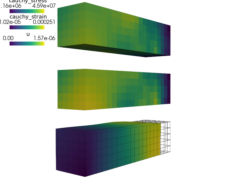
View the resulting deformation using:
color by
:python postproc.py output/ed/user_block.h5 -b --wireframe --only-names=u -d 'u,plot_displacements,rel_scaling=1e3'
color by
 :
:python postproc.py output/ed/user_block.h5 -b --wireframe --only-names=u -d 'u,plot_displacements,rel_scaling=1e3,color_kind="tensors",color_name="cauchy_strain"'
color by
 :
:python postproc.py output/ed/user_block.h5 -b --wireframe --only-names=u -d 'u,plot_displacements,rel_scaling=1e3,color_kind="tensors",color_name="cauchy_stress"'
r"""
The linear elastodynamics solution of an iron plate impact problem.

Find :math:`\ul{u}` such that:

.. math::
    \int_{\Omega} \rho \ul{v} \pddiff{\ul{u}}{\ul{v}}
    + \int_{\Omega} D_{ijkl}\ e_{ij}(\ul{v}) e_{kl}(\ul{u})
    = 0
    \;, \quad \forall \ul{v} \;,

where

.. math::
    D_{ijkl} = \mu (\delta_{ik} \delta_{jl}+\delta_{il} \delta_{jk}) +
    \lambda \ \delta_{ij} \delta_{kl}
    \;.

Notes
-----

The used elastodynamics solvers expect that the total vector of DOFs contains
three blocks in this order: the displacements, the velocities, and the
accelerations. This is achieved by defining three unknown variables ``'u'``,
``'du'``, ``'ddu'`` and the corresponding test variables, see the `variables`
definition. Then the solver can automatically extract the mass, damping (zero
here), and stiffness matrices as diagonal blocks of the global matrix. Note
also the use of the ``'dw_zero'`` (do-nothing) term that prevents the
velocity-related variables to be removed from the equations in the absence of a
damping term.

Usage Examples
--------------

Run with the default settings (the Newmark method, 3D problem, results stored
in ``output/ed/``)::

  python simple.py examples/linear_elasticity/elastodynamic.py

Solve using the Bathe method::

  python simple.py examples/linear_elasticity/elastodynamic.py -O "ts='tsb'"

View the resulting deformation using:

- color by :math:`\ul{u}`::

    python postproc.py output/ed/user_block.h5 -b --wireframe --only-names=u -d 'u,plot_displacements,rel_scaling=1e3'

- color by :math:`\ull{e}(\ul{u})`::

    python postproc.py output/ed/user_block.h5 -b --wireframe --only-names=u -d 'u,plot_displacements,rel_scaling=1e3,color_kind="tensors",color_name="cauchy_strain"'

- color by :math:`\ull{\sigma}(\ul{u})`::

    python postproc.py output/ed/user_block.h5 -b --wireframe --only-names=u -d 'u,plot_displacements,rel_scaling=1e3,color_kind="tensors",color_name="cauchy_stress"'
"""
from __future__ import absolute_import

import numpy as nm

import sfepy.mechanics.matcoefs as mc
from sfepy.discrete.fem.meshio import UserMeshIO
from sfepy.mesh.mesh_generators import gen_block_mesh

plane = 'strain'
dim = 3

# Material parameters.
E = 200e9
nu = 0.3
rho = 7800.0

lam, mu = mc.lame_from_youngpoisson(E, nu, plane=plane)
# Longitudinal and shear wave propagation speeds.
cl = nm.sqrt((lam + 2.0 * mu) / rho)
cs = nm.sqrt(mu / rho)

# Initial velocity.
v0 = 1.0

# Mesh dimensions and discretization.
d = 2.5e-3
if dim == 3:
    L = 4 * d
    dims = [L, d, d]

    shape = [21, 6, 6]
    #shape = [101, 26, 26]

else:
    L = 2 * d
    dims = [L, 2 * d]

    shape = [61, 61]
    # shape = [361, 361]

# Element size.
H = L / (shape[0] - 1)

# Time-stepping parameters.
# Note: the Courant number C0 =  dt * cl / H
dt = H / cl # C0 = 1

if dim == 3:
    t1 = 0.9 * L / cl

else:
    t1 = 1.5 * d / cl

def mesh_hook(mesh, mode):
    """
    Generate the block mesh.
    """
    if mode == 'read':
        mesh = gen_block_mesh(dims, shape, 0.5 * nm.array(dims),
                              name='user_block', verbose=False)
        return mesh

    elif mode == 'write':
        pass

def post_process(out, problem, state, extend=False):
    """
    Calculate and output strain and stress for given displacements.
    """
    from sfepy.base.base import Struct

    ev = problem.evaluate
    strain = ev('ev_cauchy_strain.i.Omega(u)', mode='el_avg', verbose=False)
    stress = ev('ev_cauchy_stress.i.Omega(solid.D, u)', mode='el_avg',
                copy_materials=False, verbose=False)

    out['cauchy_strain'] = Struct(name='output_data', mode='cell',
                                  data=strain, dofs=None)
    out['cauchy_stress'] = Struct(name='output_data', mode='cell',
                                  data=stress, dofs=None)

    return out

filename_mesh = UserMeshIO(mesh_hook)

regions = {
    'Omega' : 'all',
    'Impact' : ('vertices in (x < 1e-12)', 'facet'),
}
if dim == 3:
    regions.update({
        'Symmetry-y' : ('vertices in (y < 1e-12)', 'facet'),
        'Symmetry-z' : ('vertices in (z < 1e-12)', 'facet'),
    })

# Iron.
materials = {
    'solid' : ({
            'D': mc.stiffness_from_youngpoisson(dim=dim, young=E, poisson=nu,
                                                plane=plane),
            'rho': rho,
     },),
}

fields = {
    'displacement': ('real', 'vector', 'Omega', 1),
}

integrals = {
    'i' : 2,
}

variables = {
    'u' : ('unknown field', 'displacement', 0),
    'du' : ('unknown field', 'displacement', 1),
    'ddu' : ('unknown field', 'displacement', 2),
    'v' : ('test field', 'displacement', 'u'),
    'dv' : ('test field', 'displacement', 'du'),
    'ddv' : ('test field', 'displacement', 'ddu'),
}

ebcs = {
    'Impact' : ('Impact', {'u.0' : 0.0, 'du.0' : 0.0, 'ddu.0' : 0.0}),
}
if dim == 3:
    ebcs.update({
        'Symmtery-y' : ('Symmetry-y',
                        {'u.1' : 0.0, 'du.1' : 0.0, 'ddu.1' : 0.0}),
        'Symmetry-z' : ('Symmetry-z',
                        {'u.2' : 0.0, 'du.2' : 0.0, 'ddu.2' : 0.0}),
    })

def get_ic(coor, ic, mode='u'):
    val = nm.zeros_like(coor)
    if mode == 'u':
        val[:, 0] = 0.0

    elif mode == 'du':
        val[:, 0] = -1.0

    return val

functions = {
    'get_ic_u' : (get_ic,),
    'get_ic_du' : (lambda coor, ic: get_ic(coor, None, mode='du'),),
}

ics = {
    'ic' : ('Omega', {'u.all' : 'get_ic_u', 'du.all' : 'get_ic_du'}),
}

equations = {
    'balance_of_forces' :
    """dw_volume_dot.i.Omega(solid.rho, ddv, ddu)
     + dw_zero.i.Omega(dv, du)
     + dw_lin_elastic.i.Omega(solid.D, v, u) = 0""",
}

solvers = {
    'ls' : ('ls.scipy_direct', {
        'use_presolve' : True,
    }),
    'ls-i' : ('ls.petsc', {
        'method' : 'cg',
        'precond' : 'icc',
        'i_max' : 150,
        'eps_a' : 1e-32,
        'eps_r' : 1e-8,
        'verbose' : 2,
    }),
    'newton' : ('nls.newton', {
        'i_max'      : 1,
        'eps_a'      : 1e-6,
        'eps_r'      : 1e-6,
    }),
    'tsvv' : ('ts.velocity_verlet', {
        # Excplicit method -> requires at least 10x smaller dt than the other
        # time-stepping solvers.
        't0' : 0.0,
        't1' : t1,
        'dt' : dt,
        'n_step' : None,

        'is_linear'  : True,

        'verbose' : 1,
    }),
    'tsn' : ('ts.newmark', {
        't0' : 0.0,
        't1' : t1,
        'dt' : dt,
        'n_step' : None,

        'is_linear'  : True,

        'beta' : 0.25,
        'gamma' : 0.5,

        'verbose' : 1,
    }),
    'tsga' : ('ts.generalized_alpha', {
        't0' : 0.0,
        't1' : t1,
        'dt' : dt,
        'n_step' : None,

        'is_linear'  : True,

        'rho_inf' : 0.5,
        'alpha_m' : None,
        'alpha_f' : None,
        'beta' : None,
        'gamma' : None,

        'verbose' : 1,
    }),
    'tsb' : ('ts.bathe', {
        't0' : 0.0,
        't1' : t1,
        'dt' : dt,
        'n_step' : None,

        'is_linear'  : True,

        'verbose' : 1,
    }),
}

options = {
    'ts' : 'tsn',
    # 'ts' : 'tsb',
    'nls' : 'newton',
    # 'ls' : 'ls-i',
    'ls' : 'ls',

    'save_times' : 20,

    'active_only' : False,

    'output_format' : 'h5',
    'output_dir' : 'output/ed',
    'post_process_hook' : 'post_process',
}