diffusion/poisson_parametric_study.py
Description
Poisson equation.
This example demonstrates parametric study capabilities of Application classes. In particular (written in the strong form):

where  is a square domain,
  is
a circular domain.
is
a circular domain.
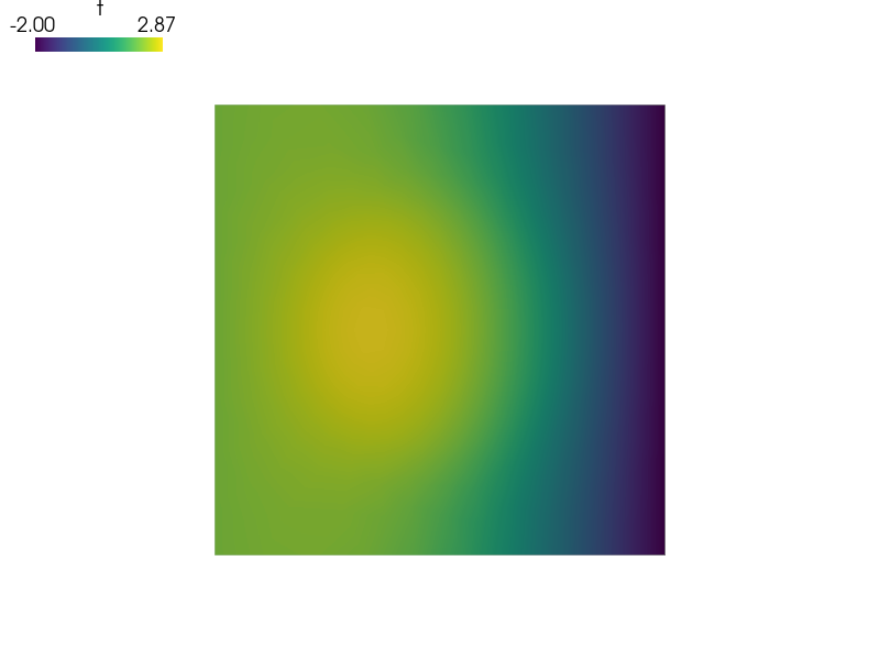
Now let’s see what happens if  diameter changes.
Run:
sfepy-run sfepy/examples/diffusion/poisson_parametric_study.py
and then look in ‘output/r_omega1’ directory, try for example:
sfepy-view output/r_omega1/circles_in_square*.vtk -2
Remark: this simple case could be achieved also by defining
by a time-dependent function and solve the static
problem as a time-dependent problem. However, the approach below is much
more general.
Find  such that:
r"""
Poisson equation.

This example demonstrates parametric study capabilities of Application
classes. In particular (written in the strong form):

.. math::
    c \Delta t = f \mbox{ in } \Omega,

    t = 2 \mbox{ on } \Gamma_1 \;,
    t = -2 \mbox{ on } \Gamma_2 \;,
    f = 1 \mbox{ in } \Omega_1 \;,
    f = 0 \mbox{ otherwise,}

where :math:`\Omega` is a square domain, :math:`\Omega_1 \in \Omega` is
a circular domain.

Now let's see what happens if :math:`\Omega_1` diameter changes.

Run::

  sfepy-run sfepy/examples/diffusion/poisson_parametric_study.py

and then look in 'output/r_omega1' directory, try for example::

  sfepy-view output/r_omega1/circles_in_square*.vtk -2

Remark: this simple case could be achieved also by defining
:math:`\Omega_1` by a time-dependent function and solve the static
problem as a time-dependent problem. However, the approach below is much
more general.

Find :math:`t` such that:

.. math::
    \int_{\Omega} c \nabla s \cdot \nabla t
    = 0
    \;, \quad \forall s \;.
"""
import os
import numpy as nm

from sfepy import data_dir
from sfepy.base.base import output

# Mesh.
filename_mesh = data_dir + '/meshes/2d/special/circles_in_square.vtk'

# Options. The value of 'parametric_hook' is the function that does the
# parametric study.
options = {
    'nls' : 'newton', # Nonlinear solver
    'ls' : 'ls', # Linear solver

    'parametric_hook' : 'vary_omega1_size',
    'output_dir' : 'output/r_omega1',
}

# Domain and subdomains.
default_diameter = 0.25
regions = {
    'Omega' : 'all',
    'Gamma_1' : ('vertices in (x < -0.999)', 'facet'),
    'Gamma_2' : ('vertices in (x > 0.999)', 'facet'),
    'Omega_1' : 'vertices by select_circ',
}

# FE field defines the FE approximation: 2_3_P1 = 2D, P1 on triangles.
field_1 = {
    'name' : 'temperature',
    'dtype' : 'real',
    'shape' : (1,),
    'region' : 'Omega',
    'approx_order' : 1,
}

# Unknown and test functions (FE sense).
variables = {
    't' : ('unknown field', 'temperature', 0),
    's' : ('test field', 'temperature', 't'),
}

# Dirichlet boundary conditions.
ebcs = {
    't1' : ('Gamma_1', {'t.0' : 2.0}),
    't2' : ('Gamma_2', {'t.0' : -2.0}),
}

# Material coefficient c and source term value f.
material_1 = {
    'name' : 'coef',
    'values' : {
        'val' : 1.0,
    }
}
material_2 = {
    'name' : 'source',
    'values' : {
        'val' : 10.0,
    }
}

# Numerical quadrature and the equation.
integral_1 = {
    'name' : 'i',
    'order' : 2,
}

equations = {
    'Poisson' : """dw_laplace.i.Omega( coef.val, s, t )
                 = dw_volume_lvf.i.Omega_1( source.val, s )"""
}

# Solvers.
solver_0 = {
    'name' : 'ls',
    'kind' : 'ls.scipy_direct',
}

solver_1 = {
    'name' : 'newton',
    'kind' : 'nls.newton',

    'i_max'      : 1,
    'eps_a'      : 1e-10,
    'eps_r'      : 1.0,
    'macheps'   : 1e-16,
    'lin_red'    : 1e-2, # Linear system error < (eps_a * lin_red).
    'ls_red'     : 0.1,
    'ls_red_warp' : 0.001,
    'ls_on'      : 1.1,
    'ls_min'     : 1e-5,
    'check'     : 0,
    'delta'     : 1e-6,
}

functions = {
    'select_circ': (lambda coors, domain=None:
                    select_circ(coors[:,0], coors[:,1], 0, default_diameter),),
}

# Functions.
def select_circ( x, y, z, diameter ):
    """Select circular subdomain of a given diameter."""
    r = nm.sqrt( x**2 + y**2 )

    out = nm.where(r < diameter)[0]

    n = out.shape[0]
    if n <= 3:
        raise ValueError( 'too few vertices selected! (%d)' % n )

    return out

def vary_omega1_size( problem ):
    r"""Vary size of \Omega1. Saves also the regions into options['output_dir'].

    Input:
      problem: Problem instance
    Return:
      a generator object:
      1. creates new (modified) problem
      2. yields the new (modified) problem and output container
      3. use the output container for some logging
      4. yields None (to signal next iteration to Application)
    """
    from sfepy.discrete import Problem
    from sfepy.solvers.ts import get_print_info

    output.prefix = 'vary_omega1_size:'

    diameters = nm.linspace( 0.1, 0.6, 7 ) + 0.001
    ofn_trunk, output_format = problem.ofn_trunk, problem.output_format
    output_dir = problem.output_dir
    join = os.path.join

    conf = problem.conf
    cf = conf.get_raw( 'functions' )
    n_digit, aux, d_format = get_print_info( len( diameters ) + 1 )
    for ii, diameter in enumerate( diameters ):
        output( 'iteration %d: diameter %3.2f' % (ii, diameter) )

        cf['select_circ'] = (lambda coors, domain=None:
                             select_circ(coors[:,0], coors[:,1], 0, diameter),)
        conf.edit('functions', cf)
        problem = Problem.from_conf(conf)

        problem.save_regions( join( output_dir, ('regions_' + d_format) % ii ),
                              ['Omega_1'] )
        region = problem.domain.regions['Omega_1']
        if not region.has_cells():
            raise ValueError('region %s has no cells!' % region.name)

        ofn_trunk = ofn_trunk + '_' + (d_format % ii)
        problem.setup_output(output_filename_trunk=ofn_trunk,
                             output_dir=output_dir,
                             output_format=output_format)

        out = []
        yield problem, out

        out_problem, state = out[-1]

        filename = join( output_dir,
                         ('log_%s.txt' % d_format) % ii )
        fd = open( filename, 'w' )
        log_item = r'$r(\Omega_1)$: %f\n' % diameter
        fd.write( log_item )
        fd.write( 'solution:\n' )
        nm.savetxt(fd, state())
        fd.close()

        yield None