large_deformation/gen_yeoh_tl_up_interactive.py
Description
Incompressible generalized Yeoh hyperelastic material model.
In this model, the deformation energy density per unit reference volume is given by

where  is the first main invariant of the deviatoric part
of the right Cauchy-Green deformation tensor
is the first main invariant of the deviatoric part
of the right Cauchy-Green deformation tensor  , the coefficients
 and exponents
  are material parameters.
Only a single term (
are material parameters.
Only a single term (dw_tl_he_genyeoh) is used in this example for
the sake of simplicity.
Components of the second Piola-Kirchhoff stress are in the case of an incompressible material
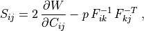
where  is the hydrostatic pressure.
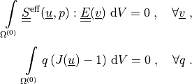
The large deformation is described using the total Lagrangian formulation in
this example. The incompressibility is treated by mixed displacement-pressure
formulation. The weak formulation is:
Find the displacement field  and pressure field
such that:
and pressure field
such that:
The following formula holds for the axial true (Cauchy) stress in the case of uniaxial stress:
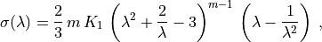
where  is the prescribed stretch (
 and
and
 being the original and deformed specimen length respectively).
The boundary conditions are set so that a state of uniaxial stress is achieved,
i.e. appropriate components of displacement are fixed on the “Left”, “Bottom”,
and “Near” faces and a monotonously increasing displacement is prescribed on
the “Right” face. This prescribed displacement is then used to calculate
 and to convert the second Piola-Kirchhoff stress to the true
(Cauchy) stress.
and to convert the second Piola-Kirchhoff stress to the true
(Cauchy) stress.
Note on material parameters
The three-term generalized Yeoh model is meant to be used for modelling of filled rubbers. The following choice of parameters is suggested [1] based on experimental data and stability considerations:
,
,
,
,
.
Usage Examples
Default options:
python3 sfepy/examples/large_deformation/gen_yeoh_tl_up_interactive.py
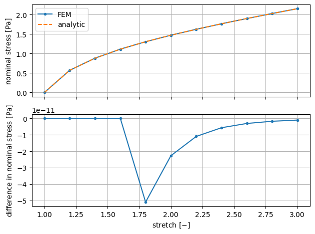
To show a comparison of stress against the analytic formula:
python3 sfepy/examples/large_deformation/gen_yeoh_tl_up_interactive.py -p
Using different mesh fineness:
python3 sfepy/examples/large_deformation/gen_yeoh_tl_up_interactive.py \
  --shape "5, 5, 5"
Different dimensions of the computational domain:
python3 sfepy/examples/large_deformation/gen_yeoh_tl_up_interactive.py \
  --dims "2, 1, 3"
Different length of time interval and/or number of time steps:
python3 sfepy/examples/large_deformation/gen_yeoh_tl_up_interactive.py \
  -t 0,15,21
Use higher approximation order (the -t option to decrease the time step is
required for convergence here):
python3 sfepy/examples/large_deformation/gen_yeoh_tl_up_interactive.py \
  --order 2 -t 0,2,21
Change material parameters:
python3 sfepy/examples/large_deformation/gen_yeoh_tl_up_interactive.py -m 2,1
View the results using sfepy-view
Show pressure on deformed mesh (use PgDn/PgUp to jump forward/back):
sfepy-view --fields=p:f1:wu:p1 domain.??.vtk
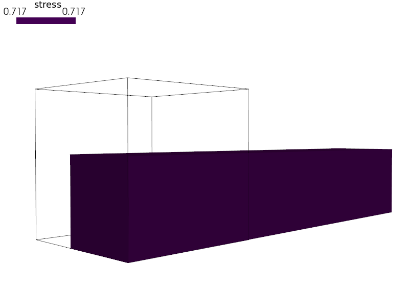
Show the axial component of stress (second Piola-Kirchhoff):
sfepy-view --fields=stress:c0 domain.??.vtk
[1] Travis W. Hohenberger, Richard J. Windslow, Nicola M. Pugno, James J. C. Busfield. Aconstitutive Model For Both Lowand High Strain Nonlinearities In Highly Filled Elastomers And Implementation With User-Defined Material Subroutines In Abaqus. Rubber Chemistry And Technology, Vol. 92, No. 4, Pp. 653-686 (2019)
#!/usr/bin/env python
r"""
Incompressible generalized Yeoh hyperelastic material model.

In this model, the deformation energy density per unit reference volume is
given by

.. math::
    W =
      K_1 \, \left( \overline I_1 - 3 \right)^{m}
      +K_2 \, \left( \overline I_1 - 3 \right)^{p}
      +K_3 \, \left( \overline I_1 - 3 \right)^{q}

where :math:`\overline I_1` is the first main invariant of the deviatoric part
of the right Cauchy-Green deformation tensor :math:`\ull{C}`, the coefficients
:math:`K_1, K_2, K_3` and exponents :math:`m, p, q` are material parameters.
Only a single term (:class:`dw_tl_he_genyeoh
<sfepy.terms.terms_hyperelastic_tl.GenYeohTLTerm>`) is used in this example for
the sake of simplicity.

Components of the second Piola-Kirchhoff stress are in the case of an
incompressible material

.. math::
    S_{ij} = 2 \, \pdiff{W}{C_{ij}} - p \, F^{-1}_{ik} \, F^{-T}_{kj} \;,

where :math:`p` is the hydrostatic pressure.

The large deformation is described using the total Lagrangian formulation in
this example. The incompressibility is treated by mixed displacement-pressure
formulation. The weak formulation is:
Find the displacement field :math:`\ul{u}` and pressure field :math:`p`
such that:

.. math::
    \intl{\Omega\suz}{} \ull{S}\eff(\ul{u}, p) : \ull{E}(\ul{v})
    \difd{V} = 0
    \;, \quad \forall \ul{v} \;,

    \intl{\Omega\suz}{} q\, (J(\ul{u})-1) \difd{V} = 0
    \;, \quad \forall q \;.

The following formula holds for the axial true (Cauchy) stress in the case of
uniaxial stress:

.. math::
    \sigma(\lambda) =
        \frac{2}{3} \, m \, K_1 \,
        \left( \lambda^2 + \frac{2}{\lambda} - 3 \right)^{m-1} \,
        \left( \lambda - \frac{1}{\lambda^2} \right) \;,

where :math:`\lambda = l/l_0` is the prescribed stretch (:math:`l_0` and
:math:`l` being the original and deformed specimen length respectively).

The boundary conditions are set so that a state of uniaxial stress is achieved,
i.e. appropriate components of displacement are fixed on the "Left", "Bottom",
and "Near" faces and a monotonously increasing displacement is prescribed on
the "Right" face. This prescribed displacement is then used to calculate
:math:`\lambda` and to convert the second Piola-Kirchhoff stress to the true
(Cauchy) stress.

Note on material parameters
---------------------------

The three-term generalized Yeoh model is meant to be used for modelling of
filled rubbers. The following choice of parameters is suggested [1] based on
experimental data and stability considerations:

  :math:`K_1 > 0`,

  :math:`K_2 < 0`,

  :math:`K_3 > 0`,

  :math:`0.7 < m < 1`,

  :math:`m < p < q`.

Usage Examples
--------------

Default options::

  python3 sfepy/examples/large_deformation/gen_yeoh_tl_up_interactive.py

To show a comparison of stress against the analytic formula::

  python3 sfepy/examples/large_deformation/gen_yeoh_tl_up_interactive.py -p

Using different mesh fineness::

  python3 sfepy/examples/large_deformation/gen_yeoh_tl_up_interactive.py \
    --shape "5, 5, 5"

Different dimensions of the computational domain::

  python3 sfepy/examples/large_deformation/gen_yeoh_tl_up_interactive.py \
    --dims "2, 1, 3"

Different length of time interval and/or number of time steps::

  python3 sfepy/examples/large_deformation/gen_yeoh_tl_up_interactive.py \
    -t 0,15,21

Use higher approximation order (the ``-t`` option to decrease the time step is
required for convergence here)::

  python3 sfepy/examples/large_deformation/gen_yeoh_tl_up_interactive.py \
    --order 2 -t 0,2,21

Change material parameters::

  python3 sfepy/examples/large_deformation/gen_yeoh_tl_up_interactive.py -m 2,1

View the results using ``sfepy-view``
-------------------------------------

Show pressure on deformed mesh (use PgDn/PgUp to jump forward/back)::

  sfepy-view --fields=p:f1:wu:p1 domain.??.vtk

Show the axial component of stress (second Piola-Kirchhoff)::

  sfepy-view --fields=stress:c0 domain.??.vtk

[1] Travis W. Hohenberger, Richard J. Windslow, Nicola M. Pugno, James J. C.
Busfield. Aconstitutive Model For Both Lowand High Strain Nonlinearities In
Highly Filled Elastomers And Implementation With User-Defined Material
Subroutines In Abaqus. Rubber Chemistry And Technology, Vol. 92, No. 4, Pp.
653-686 (2019)
"""
import argparse
import sys

SFEPY_DIR = '.'
sys.path.append(SFEPY_DIR)

import matplotlib.pyplot as plt
import numpy as np

from sfepy.base.base import IndexedStruct, Struct
from sfepy.discrete import (
    FieldVariable, Material, Integral, Function, Equation, Equations, Problem)
from sfepy.discrete.conditions import Conditions, EssentialBC
from sfepy.discrete.fem import FEDomain, Field
from sfepy.homogenization.utils import define_box_regions
from sfepy.mesh.mesh_generators import gen_block_mesh
from sfepy.solvers.ls import ScipyDirect
from sfepy.solvers.nls import Newton
from sfepy.solvers.ts_solvers import SimpleTimeSteppingSolver
from sfepy.terms import Term

DIMENSION = 3

def get_displacement(ts, coors, bc=None, problem=None):
    """
    Define the time-dependent displacement.
    """
    out = 1. * ts.time * coors[:, 0]
    return out

def _get_analytic_stress(stretches, coef, exp):
    out =  np.array([
        2 * coef * exp * (stretch**2 + 2 / stretch - 3)**(exp - 1)
        * (stretch - stretch**-2)
        if (stretch**2 + 2 / stretch > 3) else 0.
        for stretch in stretches])
    return out

def plot_graphs(
        material_parameters, global_stress, global_displacement,
        undeformed_length):
    """
    Plot a comparison of the nominal stress computed by the FEM and using the
    analytic formula.

    Parameters
    ----------
    material_parameters : list or tuple of float
        The K_1 coefficient and exponent m.
    global_displacement
        The total displacement for each time step, from the FEM.
    global_stress
        The true (Cauchy) stress for each time step, from the FEM.
    undeformed_length : float
        The length of the undeformed specimen.
    """
    coef, exp = material_parameters

    stretch = 1 + np.array(global_displacement) / undeformed_length

    # axial stress values
    stress_fem_2pk = np.array([sig for sig in global_stress])
    stress_fem = stress_fem_2pk * stretch
    stress_analytic = _get_analytic_stress(stretch, coef, exp)

    fig, (ax_stress, ax_difference) = plt.subplots(nrows=2, sharex=True)

    ax_stress.plot(stretch, stress_fem, '.-', label='FEM')
    ax_stress.plot(stretch, stress_analytic, '--', label='analytic')

    ax_difference.plot(stretch, stress_fem - stress_analytic, '.-')

    ax_stress.legend(loc='best').set_draggable(True)
    ax_stress.set_ylabel(r'nominal stress $\mathrm{[Pa]}$')
    ax_stress.grid()

    ax_difference.set_ylabel(r'difference in nominal stress $\mathrm{[Pa]}$')
    ax_difference.set_xlabel(r'stretch $\mathrm{[-]}$')
    ax_difference.grid()
    plt.tight_layout()

    return fig

def stress_strain(
        out, problem, _state, order=1, global_stress=None,
        global_displacement=None, **_):
    """
    Compute the stress and the strain and add them to the output.

    Parameters
    ----------
    out : dict
        Holds the results of the finite element computation.
    problem : sfepy.discrete.Problem
    order : int
        The approximation order of the displacement field.
    global_displacement
        Total displacement for each time step, current value will be appended.
    global_stress
        The true (Cauchy) stress for each time step, current value will be
        appended.

    Returns
    -------
    out : dict
    """
    strain = problem.evaluate(
        'dw_tl_he_genyeoh.%d.Omega(m1.par, v, u)' % (2*order),
        mode='el_avg', term_mode='strain', copy_materials=False)

    out['green_strain'] = Struct(
        name='output_data', mode='cell', data=strain, dofs=None)

    stress_1 = problem.evaluate(
        'dw_tl_he_genyeoh.%d.Omega(m1.par, v, u)' % (2*order),
        mode='el_avg', term_mode='stress', copy_materials=False)
    stress_p = problem.evaluate(
        'dw_tl_bulk_pressure.%d.Omega(v, u, p)' % (2*order),
        mode='el_avg', term_mode='stress', copy_materials=False)
    stress = stress_1 + stress_p

    out['stress'] = Struct(
        name='output_data', mode='cell', data=stress, dofs=None)

    global_stress.append(stress[0, 0, 0, 0])
    global_displacement.append(get_displacement(
        problem.ts, np.array([[1., 0, 0]]))[0])

    return out

def main(cli_args):
    dims = parse_argument_list(cli_args.dims, float)
    shape = parse_argument_list(cli_args.shape, int)
    centre = parse_argument_list(cli_args.centre, float)
    material_parameters = parse_argument_list(cli_args.material_parameters,
                                              float)
    order = cli_args.order

    ts_vals = cli_args.ts.split(',')
    ts = {
        't0' : float(ts_vals[0]), 't1' : float(ts_vals[1]),
        'n_step' : int(ts_vals[2])}

    do_plot = cli_args.plot

    ### Mesh and regions ###
    mesh = gen_block_mesh(
        dims, shape, centre, name='block', verbose=False)
    domain = FEDomain('domain', mesh)

    omega = domain.create_region('Omega', 'all')

    lbn, rtf = domain.get_mesh_bounding_box()
    box_regions = define_box_regions(3, lbn, rtf)
    regions = dict([
        [r, domain.create_region(r, box_regions[r][0], box_regions[r][1])]
        for r in box_regions])

    ### Fields ###
    scalar_field = Field.from_args(
        'fu', np.float64, 'scalar', omega, approx_order=order-1)
    vector_field = Field.from_args(
        'fv', np.float64, 'vector', omega, approx_order=order)

    u = FieldVariable('u', 'unknown', vector_field, history=1)
    v = FieldVariable('v', 'test', vector_field, primary_var_name='u')
    p = FieldVariable('p', 'unknown', scalar_field, history=1)
    q = FieldVariable('q', 'test', scalar_field, primary_var_name='p')

    ### Material ###
    coefficient, exponent  = material_parameters
    m_1 = Material(
        'm1', par=[coefficient, exponent],
    )

    ### Boundary conditions ###
    x_sym = EssentialBC('x_sym', regions['Left'], {'u.0' : 0.0})
    y_sym = EssentialBC('y_sym', regions['Near'], {'u.1' : 0.0})
    z_sym = EssentialBC('z_sym', regions['Bottom'], {'u.2' : 0.0})
    disp_fun = Function('disp_fun', get_displacement)
    displacement = EssentialBC(
        'displacement', regions['Right'], {'u.0' : disp_fun})
    ebcs = Conditions([x_sym, y_sym, z_sym, displacement])

    ### Terms and equations ###
    integral = Integral('i', order=2*order+1)

    term_1 = Term.new(
        'dw_tl_he_genyeoh(m1.par, v, u)',
        integral, omega, m1=m_1, v=v, u=u)
    term_pressure = Term.new(
        'dw_tl_bulk_pressure(v, u, p)',
        integral, omega, v=v, u=u, p=p)

    term_volume_change = Term.new(
        'dw_tl_volume(q, u)',
        integral, omega, q=q, u=u, term_mode='volume')
    term_volume = Term.new(
        'dw_integrate(q)',
        integral, omega, q=q)

    eq_balance = Equation('balance', term_1 + term_pressure)
    eq_volume = Equation('volume', term_volume_change - term_volume)
    equations = Equations([eq_balance, eq_volume])

    ### Solvers ###
    ls = ScipyDirect({})
    nls_status = IndexedStruct()
    nls = Newton(
        {'i_max' : 20},
        lin_solver=ls, status=nls_status
    )

    ### Problem ###
    pb = Problem('hyper', equations=equations)
    pb.set_bcs(ebcs=ebcs)
    pb.set_ics(ics=Conditions([]))
    tss = SimpleTimeSteppingSolver(ts, nls=nls, context=pb)
    pb.set_solver(tss)

    ### Solution ###
    axial_stress = []
    axial_displacement = []
    def stress_strain_fun(*args, **kwargs):
        return stress_strain(
            *args, order=order, global_stress=axial_stress,
            global_displacement=axial_displacement, **kwargs)

    pb.solve(save_results=True, post_process_hook=stress_strain_fun)

    if do_plot:
        fig = plot_graphs(
            material_parameters, axial_stress, axial_displacement,
            undeformed_length=dims[0])

        fig.savefig('gen_yeoh_tl_up_comparison.png', bbox_inches='tight')

        if cli_args.show:
            plt.show()

def parse_argument_list(cli_arg, type_fun=None, value_separator=','):
    """
    Split the command-line argument into a list of items of given type.

    Parameters
    ----------
    cli_arg : str
    type_fun : function
        A function to be called on each substring of `cli_arg`; default: str.
    value_separator : str
    """
    if type_fun is None:
        type_fun = str
    out = [type_fun(value) for value in cli_arg.split(value_separator)]
    return out

def parse_args():
    """Parse command line arguments."""
    parser = argparse.ArgumentParser(
        description=__doc__,
        formatter_class=argparse.RawDescriptionHelpFormatter)
    parser.add_argument(
        '--order', type=int, default=1, help='The approximation order of the '
        'displacement field [default: %(default)s]')
    parser.add_argument(
        '-m', '--material-parameters', default='0.5, 0.9',
        help='Material parameters - coefficient and exponent - of a single '
        'term of the generalized Yeoh hyperelastic model. '
        '[default: %(default)s]')
    parser.add_argument(
        '--dims', default="1.0, 1.0, 1.0",
        help='Dimensions of the block [default: %(default)s]')
    parser.add_argument(
        '--shape', default='2, 2, 2',
        help='Shape (counts of nodes in x, y, z) of the block [default: '
        '%(default)s]')
    parser.add_argument(
        '--centre', default='0.5, 0.5, 0.5',
        help='Centre of the block [default: %(default)s]')
    parser.add_argument(
        '-p', '--plot', action='store_true', default=False,
        help='Whether to plot a comparison with analytical formula.')
    parser.add_argument(
        '-n', '--no-show', dest='show', action='store_false', default=True,
        help='Do not show matplotlib figures.')
    parser.add_argument(
        '-t', '--ts',
        type=str, default='0.0,2.0,11',
        help='Start time, end time, and number of time steps [default: '
        '"%(default)s"]')
    return parser.parse_args()

if __name__ == '__main__':
    args = parse_args()
    main(args)