diffusion/poisson_neumann.py
Description
The Poisson equation with Neumann boundary conditions on a part of the boundary.
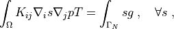
Find  such that:
where  is the given flux,
  , and
, and  (an isotropic medium). See the
tutorial section Strong form of Poisson’s equation and its integration for a detailed explanation.
(an isotropic medium). See the
tutorial section Strong form of Poisson’s equation and its integration for a detailed explanation.
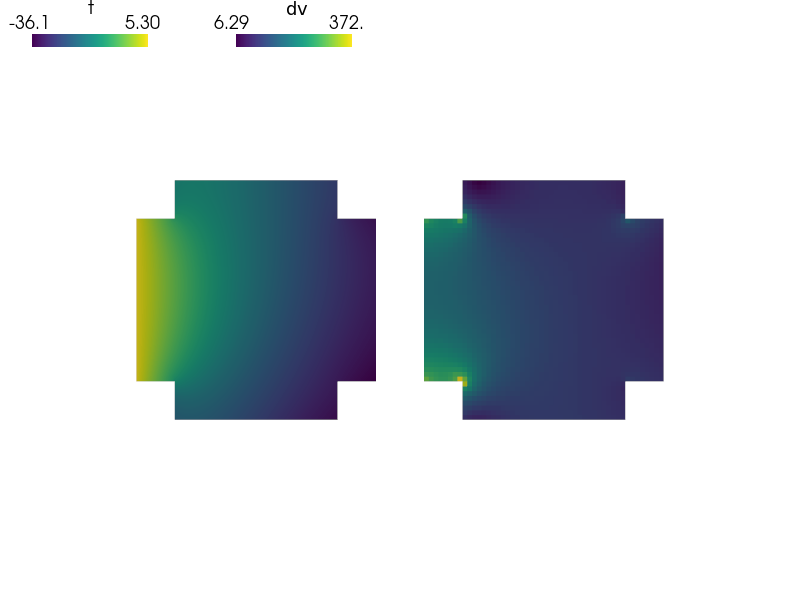
The diffusion velocity and fluxes through various parts of the boundary are
computed in the post_process() function. On ‘Gamma_N’ (the Neumann
condition boundary part), the flux/length should correspond to the given value
 , while on ‘Gamma_N0’ the flux should be zero. Use the
‘refinement_level’ option (see the usage examples below) to check the
convergence of the numerical solution to those values. The total flux and the
flux through ‘Gamma_D’ (the Dirichlet condition boundary part) are shown as
well.
, while on ‘Gamma_N0’ the flux should be zero. Use the
‘refinement_level’ option (see the usage examples below) to check the
convergence of the numerical solution to those values. The total flux and the
flux through ‘Gamma_D’ (the Dirichlet condition boundary part) are shown as
well.
Usage Examples
Run with the default settings (no refinement):
sfepy-run sfepy/examples/diffusion/poisson_neumann.py
Refine the mesh twice:
sfepy-run sfepy/examples/diffusion/poisson_neumann.py -O "'refinement_level' : 2"
r"""
The Poisson equation with Neumann boundary conditions on a part of the
boundary.

Find :math:`T` such that:

.. math::
    \int_{\Omega} K_{ij} \nabla_i s \nabla_j p T
    = \int_{\Gamma_N} s g
    \;, \quad \forall s \;,

where :math:`g` is the given flux, :math:`g = \ul{n} \cdot K_{ij} \nabla_j
\bar{T}`, and :math:`K_{ij} = c \delta_{ij}` (an isotropic medium). See the
tutorial section :ref:`poisson-weak-form-tutorial` for a detailed explanation.

The diffusion velocity and fluxes through various parts of the boundary are
computed in the :func:`post_process()` function. On 'Gamma_N' (the Neumann
condition boundary part), the flux/length should correspond to the given value
:math:`g = -50`, while on 'Gamma_N0' the flux should be zero. Use the
'refinement_level' option (see the usage examples below) to check the
convergence of the numerical solution to those values. The total flux and the
flux through 'Gamma_D' (the Dirichlet condition boundary part) are shown as
well.

Usage Examples
--------------

Run with the default settings (no refinement)::

  sfepy-run sfepy/examples/diffusion/poisson_neumann.py

Refine the mesh twice::

  sfepy-run sfepy/examples/diffusion/poisson_neumann.py -O "'refinement_level' : 2"
"""
import numpy as nm

from sfepy.base.base import output, Struct
from sfepy import data_dir

def post_process(out, pb, state, extend=False):
    """
    Calculate :math:`\nabla t` and compute boundary fluxes.
    """
    dv = pb.evaluate('ev_diffusion_velocity.i.Omega(m.K, t)', mode='el_avg',
                     verbose=False)
    out['dv'] = Struct(name='output_data', mode='cell',
                       data=dv, dofs=None)

    totals = nm.zeros(3)
    for gamma in ['Gamma_N', 'Gamma_N0', 'Gamma_D']:

        flux = pb.evaluate('ev_surface_flux.i.%s(m.K, t)' % gamma,
                           verbose=False)
        area = pb.evaluate('ev_volume.i.%s(t)' % gamma, verbose=False)

        flux_data = (gamma, flux, area, flux / area)
        totals += flux_data[1:]

        output('%8s flux: % 8.3f length: % 8.3f flux/length: % 8.3f'
               % flux_data)

    totals[2] = totals[0] / totals[1]
    output('   total flux: % 8.3f length: % 8.3f flux/length: % 8.3f'
           % tuple(totals))

    return out

filename_mesh = data_dir + '/meshes/2d/cross-51-0.34.mesh'

materials = {
    'flux' : ({'val' : -50.0},),
    'm' : ({'K' : 2.7 * nm.eye(2)},),
}

regions = {
    'Omega' : 'all',
    'Gamma_D' : ('vertices in (x < -0.4999)', 'facet'),
    'Gamma_N0' : ('vertices in (y > 0.4999)', 'facet'),
    'Gamma_N' : ('vertices of surface -s (r.Gamma_D +v r.Gamma_N0)',
                 'facet'),
}

fields = {
    'temperature' : ('real', 1, 'Omega', 1),
}

variables = {
    't' : ('unknown field', 'temperature', 0),
    's' : ('test field',    'temperature', 't'),
}

ebcs = {
    't1' : ('Gamma_D', {'t.0' : 5.3}),
}

integrals = {
    'i' : 2
}

equations = {
    'Temperature' : """
           dw_diffusion.i.Omega(m.K, s, t)
         = dw_integrate.i.Gamma_N(flux.val, s)
    """
}

solvers = {
    'ls' : ('ls.scipy_direct', {}),
    'newton' : ('nls.newton', {
        'i_max' : 1,
        'eps_a' : 1e-10,
    }),
}

options = {
    'nls' : 'newton',
    'ls' : 'ls',

    'refinement_level' : 0,
    'post_process_hook' : 'post_process',
}