Notes on solving PDEs by the Finite Element Method
The Finite Element Method (FEM) is the numerical method for solving Partial Differential Equations (PDEs). FEM was developed in the middle of XX. century and now it is widely used in different areas of science and engineering, including mechanical and structural design, biomedicine, electrical and power design, fluid dynamics and other. FEM is based on a very elegant mathematical theory of weak solution of PDEs. In this section we will briefly discuss basic ideas underlying FEM.
Strong form of Poisson’s equation and its integration
Let us start our discussion about FEM with the strong form of Poisson’s equation
(1)
(2)
(3)
where  is the solution domain with the
boundary
is the solution domain with the
boundary  ,
,  is the part of the boundary
where Dirichlet boundary conditions are given,
is the part of the boundary
where Dirichlet boundary conditions are given,  is the part of
the boundary where Neumann boundary conditions are given,
is the part of
the boundary where Neumann boundary conditions are given,  is the
unknown function to be found,
is the
unknown function to be found,  are known functions.
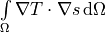
FEM is based on a weak formulation. The weak form of the equation (1) is
where  is a test function. Integrating this equation by parts
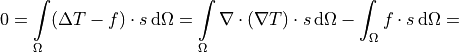
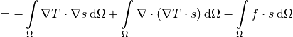
and applying Gauss theorem we obtain:
or
The surface integral term can be split into two integrals, one over the Dirichlet part of the surface and second over the Neumann part
(4)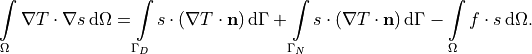
The equation (4) is the initial weak form of the Poisson’s problem (1)–(3). But we can not work with it without applying the boundary conditions. So it is time to talk about the boundary conditions.
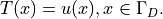
Dirichlet Boundary Conditions
On the Dirichlet part of the surface we have two restrictions. One is the Dirichlet
boundary conditions  as they are, and the second is the
integral term over in equation (4). To be
consistent we have to use only the Dirichlet conditions and avoid the integral
term. To implement this we can take the function
as they are, and the second is the
integral term over in equation (4). To be
consistent we have to use only the Dirichlet conditions and avoid the integral
term. To implement this we can take the function  and
the test function
and
the test function  , where

In other words the unknown function  must be continuous together with
its gradient in the domain. In contrast the test function must be
also continuous together with its gradient in the domain but it should be zero
on the surface .
must be continuous together with
its gradient in the domain. In contrast the test function must be
also continuous together with its gradient in the domain but it should be zero
on the surface .
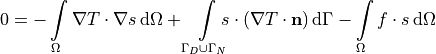
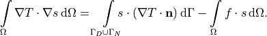
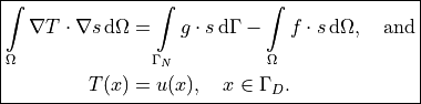
With this requirement the integral term over Dirichlet part of the surface
is vanishing and the weak form of the Poisson equation for
and becomes
That is why Dirichlet conditions in FEM terminology are called Essential Boundary Conditions. These conditions are not a part of the weak form and they are used as they are.
Neumann Boundary Conditions
The Neumann boundary conditions correspond to the known flux
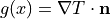 . The integral term over the Neumann
surface in the equation (4) contains exactly the same flux.
So we can use the known function
. The integral term over the Neumann
surface in the equation (4) contains exactly the same flux.
So we can use the known function  in the integral term:
where test function also belongs to the space  .
.
That is why Neumann conditions in FEM terminology are called Natural Boundary Conditions. These conditions are a part of weak form terms.
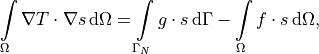
The weak form of the Poisson’s equation
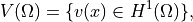
Now we can write the resulting weak form for the Poisson’s problem
(1)–(3). For any test function
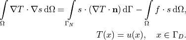
find
such that
(5)
Discussion of discretization and meshing
It is planned to have an example of the discretization based on the Poisson’s equation weak form (5). For now, please refer to the wikipedia page Finite Element Method for a basic description of the disretization and meshing.
Numerical solution of the problem
To solve numerically given problem based on the weak form (5) we have to go through 5 steps:
Define geometry of the domain
 and
surfaces and .
and
surfaces and .Define the known functions
 ,
,  and
and  .
.Define the unknown function
and the test functions .Define essential boundary conditions (Dirichlet conditions)
Define equation and natural boundary conditions (Neumann conditions) as the set of all integral terms
 ,
,
 ,
,
 .
.