Implementation of Essential Boundary Conditions
The essential boundary conditions can be applied in several ways. Here we describe the implementation used in SfePy.
Motivation
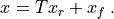
Let us solve a linear system  with
with  matrix
 with
with  values in the
  vector known. The known
values can be for example EBC values on a boundary, if comes from a
PDE discretization. If we put the known fixed values into a vector
vector known. The known
values can be for example EBC values on a boundary, if comes from a
PDE discretization. If we put the known fixed values into a vector  ,
that has the same size as , and has zeros in positions that are not
fixed, we can easily construct a
,
that has the same size as , and has zeros in positions that are not
fixed, we can easily construct a  matrix
  that
maps the reduced vector
that
maps the reduced vector  of size
  , where the
fixed values are removed, to the full vector :
, where the
fixed values are removed, to the full vector :
With that the reduced linear system with a  can be
formed:
can be
formed:
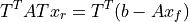
that can be solved by a linear solver. We can see, that the (non-zero) known values are now on the right-hand side of the linear system. When the known values are all zero, we have simply
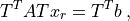
which is convenient, as it allows simply throwing away the A and b entries corresponding to the known values already during the finite element assembling.
Implementation
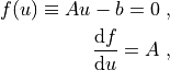
All PDEs in SfePy are solved in a uniform way as a system of non-linear equations

where  is the nonlinear function and
  the vector of unknown
DOFs. This system is solved iteratively by the Newton method
the vector of unknown
DOFs. This system is solved iteratively by the Newton method
until a convergence criterion is met. Each iteration involves solution of the system of linear equations

where the tangent matrix  and the residual
  are
are

Then
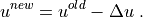
If the initial (old) vector  contains the values of EBCs at
correct positions, the increment
contains the values of EBCs at
correct positions, the increment  is zero at those
positions. This allows us to assemble directly the reduced matrix
is zero at those
positions. This allows us to assemble directly the reduced matrix  , the right-hand side
  , and ignore the values of EBCs during
assembling. The EBCs are satisfied automatically by applying them to the
initial guess
, and ignore the values of EBCs during
assembling. The EBCs are satisfied automatically by applying them to the
initial guess  , that is given to the Newton solver.
Linear Problems
For linear problems we have
and so the Newton method converges in a single iteration:

Evaluation of Residual and Tangent Matrix
The evaluation of the residual as well as the tangent matrix
within the Newton solver proceeds in the following steps:
The EBCs are applied to the full DOF vector
.The reduced vector
 is passed to the Newton solver.
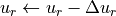
Newton iteration loop:
Evaluation of
 or
or  :
:- is reconstructed from ;
local element contributions are evaluated using
;local element contributions are assembled into
or
- values corresponding to fixed DOF positions are thrown
away.
The reduced system
 is solved.
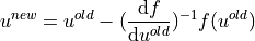
Solution is updated:
 .
.The loop is terminated if a stopping condition is satisfied, the solver returns the final
.
The final
is reconstructed from .