User’s Guide¶

This manual provides reference documentation to fish_heart from a user’s perspective.

Geometry¶

An idealized fish heart (a sphere) geometry is considered for the moment.

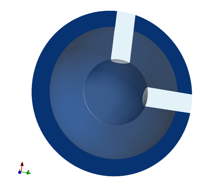
The finite element mesh and subdomains.

Due to symmetry, only a half of the domain is used.

Regions¶

The whole domain $\Omega$ is divided into the following subdomains (or regions is SfePy naming conventions), roughly corresponding to the true physiological regions:

volumes:
- inner layer (light blue) domain $\Omega_1$ containing the highly porous tissue able to suck in and out a significant volume of blood - the spongious myocardium;
- outer layer (dark blue) domain $\Omega_2$ containing the tissue with active muscle fibres - the compact myocardium;
- the domains of blood vessels (white) for blood flowing in (sinus venosus) or out (aorta) $\Omega_1$ , $\Omega_4$ (ignored in the current version);
surfaces:
- the inner surface $\Gamma_0$ ;
- the interface $\Gamma_1$ between $\Omega_1$ , $\Omega_2$ ;
- the outer surface $\Gamma_2$ ;
- the plane of symmetry $\Gamma_S$ ;
points:
- a node $A$ at $[2.481935 0.000000 0.300000]$ ;
- a node $B$ at $[0.000000 2.481935 0.300000]$ .

Fibre Directions¶

We assume an ad-hoc orientation of the muscle fibres in $\Omega_2$ , as the real orientation is not know to us. Initial quantitative microscopy studies indicate that it could be considered isotropic in the first approximation. This motivated our simple choice: two systems of fibres, one corresponding to meridians, the other to parallels, see Fig. The two systems of active muscle fibres..

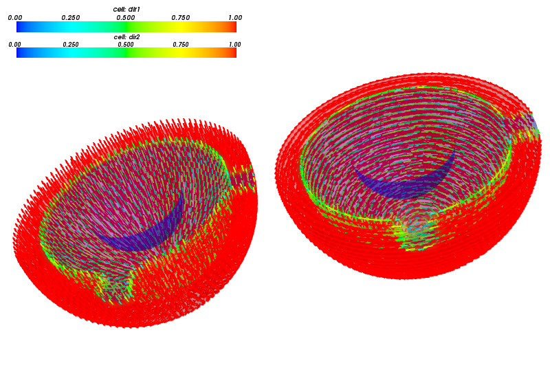
The two systems of active muscle fibres.

Mathematical Model¶

The mathematical model presented below is a custom version of the models developed by the authors for quite a long time, first introduced in a journal publication already in [rohan-cimrman-2002]. More recent publications are [cimrman-rohan-2007] and [cimrman-rohan-2009]. A detailed description of our approach to mathematical modelling of biological tissues is given in the Ph.D. thesis of R. Cirmman [cimrman-2002].

The large deformations of the tissue are described using the total Lagrangian (TL) formulation.

To study time-dependent problems the solution is advanced by $\dt$ in discrete time steps $0, 1, \dots$ . The backward difference can be used to discretize time derivatives (denoted by a dot). We also assume a quasistatic case, as inertial effects can be neglected when dealing with biological tissues. Then the solution up to the step $n-1$ is known and we seek the solution at the step $n$ satisfying the equilibrium equation and the mass balance equations. In what follows we omit the superscript $n$ and denote only the linearized values by the superscript $n-1$ .

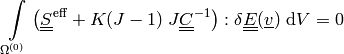
Equations in $\Omega_1$ correspond to a model developed in [cimrman-rohan-2007], restricted to one channel system only:

equilibrium equation:

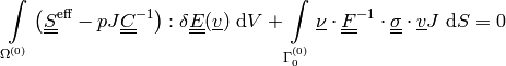
(1) $\intl{\Omega\suz}{} \left( \ull{S}\eff - p J \ull{C}^{-1} \right) : \delta \ull{E}(\ul{v}) \difd{V} + \intl{\Gamma_0\suz}{} \ul{\nu} \cdot \ull{F}^{-1} \cdot \ull{\sigma} \cdot \ul{v} J \difd{S} = 0$

where $\ull{\sigma}(t) = \pi(t) \ull{I}$ is a given pressure traction.
mass balance equation (perfusion):

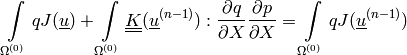
(2) $\intl{\Omega\suz}{} q J(\ul{u}) + \intl{\Omega\suz}{} \ull{K}(\ul{u}\sunm) : \pdiff{q}{X} \pdiff{p}{X} = \intl{\Omega\suz}{} q J(\ul{u}\sunm)$

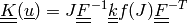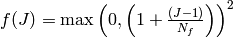The linearized deformation-dependent permeability is defined as $\ull{K}(\ul{u}) = J \ull{F}^{-1} \ull{k} f(J) \ull{F}^{-T}$ , where $\ul{u}$ relates to the previous time step $(n-1)$ and $f(J) = \max\left(0, \left(1 + \frac{(J - 1)}{N_f}\right)\right)^2$ expresses the dependence on volume compression/expansion, see Fig. The dependence of permeability on volume compression/expansion..

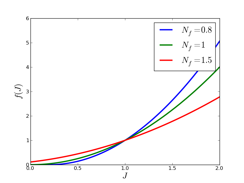
The dependence of permeability on volume compression/expansion.

Equations in $\Omega_2$ :

equilibrium equation:

(3) $\intl{\Omega\suz}{} \left( \ull{S}\eff + K(J-1)\; J \ull{C}^{-1} \right) : \delta \ull{E}(\ul{v}) \difd{V} = 0$

Near-incompressibility is treated by setting $p = - K (J - 1)$ , so there is no a separate mass balance equation like (2).

The effective stress $\ull{S}\eff$ incorporates also the effects of the active muscle fibres, cf. [rohan-cimrman-2002]. It is defined as

(4) $\ull{S}\eff = \phi_m \mu J^{-\frac{2}{3}}(\ull{I} - \frac{1}{3}\tr(\ull{C}) \ull{C}^{-1}) + \sum_{k=1}^2 \phi_f^k \tau^k \ull{\omega}^k \;,$

where the first term is the neo-Hookean term and the sum add contributions of the two fibre systems. The volume fraction satisfy $\phi_m + \sum_{k=1}^2 \phi_f^k = 1$ . The tensors $\ull{\omega}^k = \ul{d}^k\ul{d}^k$ are defined by the fibre system direction vectors $\ul{d}^k$ (unit), see Fig. The two systems of active muscle fibres..

For the one-dimensional tensions $\tau^k$ holds simply ( $^k$ omitted):

(5) $\tau = A f_{\rm max} \exp{\left\{-(\frac{\epsilon - \varepsilon_{\rm opt}}{s})^2\right\}} \mbox{ , } \epsilon = \ull{E} : \ull{\omega}$

Boundary Conditions and Loads¶

Dirichlet boundary conditions:

displacements:
- $u_3 = 0$ in the plane of symmetry $\Gamma_S$
- $u_1 = u_2 = 0$ in A, $u_1 = 0$ in B (fix rigid body modes)
pressure:
- $p = \bar{p}(t)$ on $\Gamma_0$
pressure traction load:
- $\pi(t)$ on $\Gamma_0$
fibre activation:
- given $A(t)$ in $\Omega_2$ for each system of the active fibres

See Fig. The fibre activations and pressure boundary conditions. for examples of time-dependent loads.

Numerical Simulations¶

The above model is discretized using the FEM and implemented into SfePy.

Convergence and Load Logs¶

Due to nonlinearity of the problem (1)-(5), each time step is solved by the Newton method. To have an idea about its convergence we log the error in all iterations, as can be seen in Fig. The convergence of the Newton solver in all iterations..

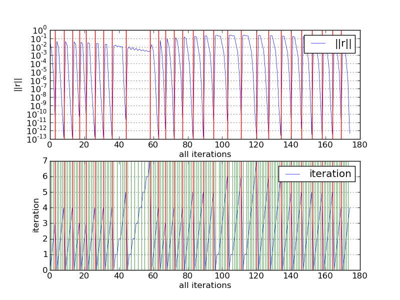
The convergence of the Newton solver in all iterations.

The individual time steps are separated by red vertical lines. Top: the error (rezidual norm). Bottom: number of iterations, green vertical lines indicate the Newton iterations; stagnations of the blue line mark a line search occurrence (= several rezidual evaluations in a single step).

Similarly, we log also the loads at each time step, see Fig. The fibre activations and pressure boundary conditions..

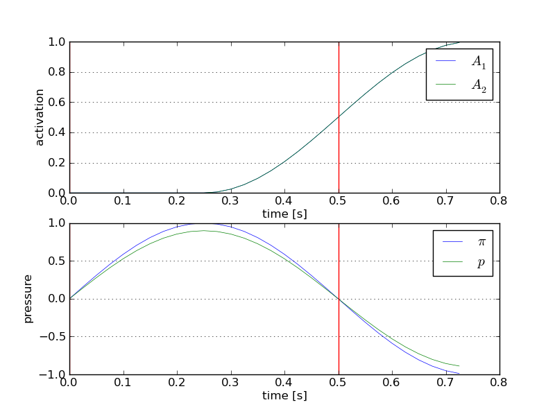
The fibre activations and pressure boundary conditions.

Preliminary Results¶

The following figures serve only as an illustration of possibilities. They were obtained using completely ad hoc material, geometrical and other parameters as a proof of concept and a test that the code could handle the real problem.

An example movie showing several quantities of interest evolving in time.
Example figures, visualized using Mayavi API.

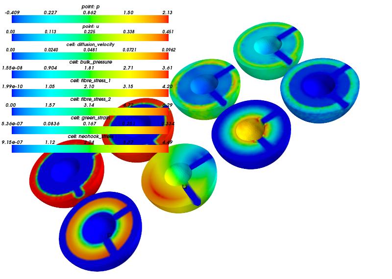
A snapshot of a single time step.

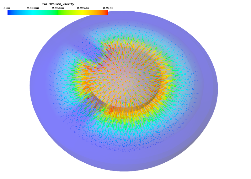
Blood flowing into the spongious myocardium during diastole.

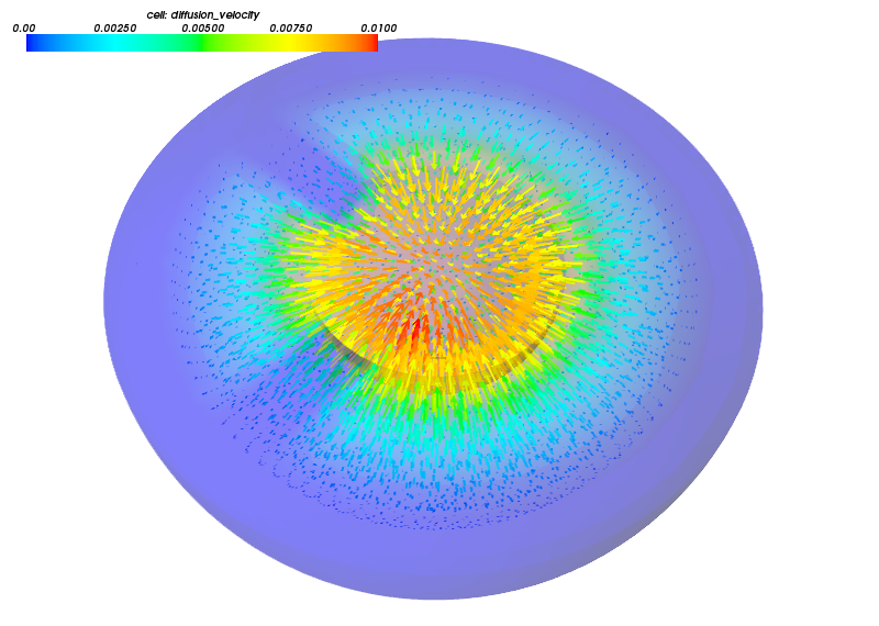
Blood flowing out of the spongious myocardium during systole.

[cimrman-2002]

Robert Cimrman (2002), Mathematical modelling of biological tissues, Ph.D. thesis, University of West Bohemia, Faculty of Applied Sciences, Department of Mechanics (link) (pdf)

[cimrman-rohan-2009]

Robert Cimrman, Eduard Rohan, On identification of the arterial model parameters from experiments applicable ‘in vivo’, Mathematics and Computers in Simulation, In Press, Corrected Proof, Available online 25 February 2009, ISSN 0378-4754, DOI: 10.1016/j.matcom.2009.02.006. (link)

[cimrman-rohan-2007]

(1, 2) Robert Cimrman, Eduard Rohan (2007), On modelling the parallel diffusion flow in deforming porous media, Mathematics and Computers in Simulation, Volume 76, Issues 1-3, Pages 34-43, ISSN 0378-4754, DOI: 10.1016/j.matcom.2007.01.034. (link)

[rohan-cimrman-2002]

(1, 2) Eduard Rohan, Robert Cimrman (2002) Sensitivity analysis and material identification for activated smooth muscle, 519-541. In Computer Assisted Mechanics and Engineering Science.

User’s Guide¶

Geometry¶

Regions¶

Fibre Directions¶

Mathematical Model¶

Boundary Conditions and Loads¶

Numerical Simulations¶

Convergence and Load Logs¶

Preliminary Results¶

Table Of Contents

Previous topic

Next topic

This Page

Navigation

User’s Guide¶

Geometry¶

Regions¶

Fibre Directions¶

Mathematical Model¶

Boundary Conditions and Loads¶

Numerical Simulations¶

Convergence and Load Logs¶

Preliminary Results¶

Table Of Contents

Previous topic

Next topic

This Page

Quick search

Navigation