large_deformation/hyperelastic.py
Description
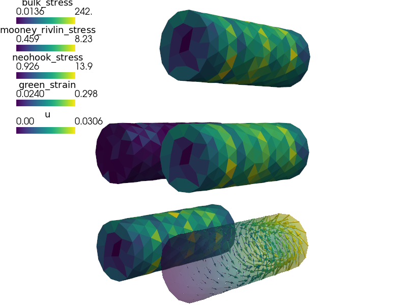
Nearly incompressible Mooney-Rivlin hyperelastic material model.
Large deformation is described using the total Lagrangian formulation. Models of this kind can be used to model e.g. rubber or some biological materials.
Find  such that:
where
|
deformation gradient |
|
|
|
right Cauchy-Green deformation tensor |
|
Green strain tensor |
|
effective second Piola-Kirchhoff stress tensor |


The effective stress  is given by:

# -*- coding: utf-8 -*-
r"""
Nearly incompressible Mooney-Rivlin hyperelastic material model.
Large deformation is described using the total Lagrangian formulation.
Models of this kind can be used to model e.g. rubber or some biological
materials.
Find :math:`\ul{u}` such that:
.. math::
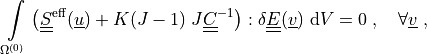
\intl{\Omega\suz}{} \left( \ull{S}\eff(\ul{u})
+ K(J-1)\; J \ull{C}^{-1} \right) : \delta \ull{E}(\ul{v}) \difd{V}
= 0
\;, \quad \forall \ul{v} \;,
where
.. list-table::
:widths: 20 80
* - :math:`\ull{F}`
- deformation gradient :math:`F_{ij} = \pdiff{x_i}{X_j}`
* - :math:`J`
- :math:`\det(F)`
* - :math:`\ull{C}`
- right Cauchy-Green deformation tensor :math:`C = F^T F`
* - :math:`\ull{E}(\ul{u})`
- Green strain tensor :math:`E_{ij} = \frac{1}{2}(\pdiff{u_i}{X_j} +
\pdiff{u_j}{X_i} + \pdiff{u_m}{X_i}\pdiff{u_m}{X_j})`
* - :math:`\ull{S}\eff(\ul{u})`
- effective second Piola-Kirchhoff stress tensor
The effective stress :math:`\ull{S}\eff(\ul{u})` is given by:
.. math::
\ull{S}\eff(\ul{u}) = \mu J^{-\frac{2}{3}}(\ull{I}
- \frac{1}{3}\tr(\ull{C}) \ull{C}^{-1})
+ \kappa J^{-\frac{4}{3}} (\tr(\ull{C}\ull{I} - \ull{C}
- \frac{2}{6}((\tr{\ull{C}})^2 - \tr{(\ull{C}^2)})\ull{C}^{-1})
\;.
"""
import numpy as nm
from sfepy import data_dir
filename_mesh = data_dir + '/meshes/3d/cylinder.mesh'
options = {
'nls' : 'newton',
'ls' : 'ls',
'ts' : 'ts',
'save_times' : 'all',
'post_process_hook' : 'stress_strain',
}
field_1 = {
'name' : 'displacement',
'dtype' : nm.float64,
'shape' : 3,
'region' : 'Omega',
'approx_order' : 1,
}
material_1 = {
'name' : 'solid',
'values' : {
'K' : 1e3, # bulk modulus
'mu' : 20e0, # shear modulus of neoHookean term
'kappa' : 10e0, # shear modulus of Mooney-Rivlin term
}
}
variables = {
'u' : ('unknown field', 'displacement', 0),
'v' : ('test field', 'displacement', 'u'),
}
regions = {
'Omega' : 'all',
'Left' : ('vertices in (x < 0.001)', 'facet'),
'Right' : ('vertices in (x > 0.099)', 'facet'),
}
##
# Dirichlet BC + related functions.
ebcs = {
'l' : ('Left', {'u.all' : 0.0}),
'r' : ('Right', {'u.0' : 0.0, 'u.[1,2]' : 'rotate_yz'}),
}
centre = nm.array( [0, 0], dtype = nm.float64 )
def rotate_yz(ts, coor, **kwargs):
from sfepy.linalg import rotation_matrix2d
vec = coor[:,1:3] - centre
angle = 10.0 * ts.step
print('angle:', angle)
mtx = rotation_matrix2d( angle )
vec_rotated = nm.dot( vec, mtx )
displacement = vec_rotated - vec
return displacement
functions = {
'rotate_yz' : (rotate_yz,),
}
def stress_strain( out, problem, state, extend = False ):
from sfepy.base.base import Struct, debug
ev = problem.evaluate
strain = ev('dw_tl_he_neohook.i.Omega( solid.mu, v, u )',
mode='el_avg', term_mode='strain')
out['green_strain'] = Struct(name='output_data',
mode='cell', data=strain, dofs=None)
stress = ev('dw_tl_he_neohook.i.Omega( solid.mu, v, u )',
mode='el_avg', term_mode='stress')
out['neohook_stress'] = Struct(name='output_data',
mode='cell', data=stress, dofs=None)
stress = ev('dw_tl_he_mooney_rivlin.i.Omega( solid.kappa, v, u )',
mode='el_avg', term_mode='stress')
out['mooney_rivlin_stress'] = Struct(name='output_data',
mode='cell', data=stress, dofs=None)
stress = ev('dw_tl_bulk_penalty.i.Omega( solid.K, v, u )',
mode='el_avg', term_mode= 'stress')
out['bulk_stress'] = Struct(name='output_data',
mode='cell', data=stress, dofs=None)
return out
##
# Balance of forces.
integral_1 = {
'name' : 'i',
'order' : 1,
}
equations = {
'balance' : """dw_tl_he_neohook.i.Omega( solid.mu, v, u )
+ dw_tl_he_mooney_rivlin.i.Omega( solid.kappa, v, u )
+ dw_tl_bulk_penalty.i.Omega( solid.K, v, u )
= 0""",
}
##
# Solvers etc.
solver_0 = {
'name' : 'ls',
'kind' : 'ls.scipy_direct',
}
solver_1 = {
'name' : 'newton',
'kind' : 'nls.newton',
'i_max' : 5,
'eps_a' : 1e-10,
'eps_r' : 1.0,
'macheps' : 1e-16,
'lin_red' : 1e-2, # Linear system error < (eps_a * lin_red).
'ls_red' : 0.1,
'ls_red_warp': 0.001,
'ls_on' : 1.1,
'ls_min' : 1e-5,
'check' : 0,
'delta' : 1e-6,
}
solver_2 = {
'name' : 'ts',
'kind' : 'ts.simple',
't0' : 0,
't1' : 1,
'dt' : None,
'n_step' : 11, # has precedence over dt!
'verbose' : 1,
}