large_deformation/balloon.py
Description
Inflation of a Mooney-Rivlin hyperelastic balloon.
This example serves as a verification of the membrane term (dw_tl_membrane,
TLMembraneTerm)
implementation.
Following Rivlin 1952 and Dumais, the analytical relation between a
relative stretch  of a thin (membrane) sphere made of the
Mooney-Rivlin material of the undeformed radius
of a thin (membrane) sphere made of the
Mooney-Rivlin material of the undeformed radius  , membrane
thickness
, membrane
thickness  and the inner pressure
  is
is
where  ,
,  are the Mooney-Rivlin material parameters.
In the equations below, only the surface of the domain is mechanically
important - a stiff 2D membrane is embedded in the 3D space and coincides with
the balloon surface. The volume is very soft, to simulate a fluid-filled
cavity. A similar model could be used to model e.g. plant cells. The balloon
surface is loaded by prescribing the inner volume change  .
The fluid pressure in the cavity is a single scalar value, enforced either by
the
.
The fluid pressure in the cavity is a single scalar value, enforced either by
the 'integral_mean_value' linear combination condition, when use_lcbcs
argument of define() is set to True (default), or by the
 constant approximation.
Find  and a constant such that:
balance of forces:
![\intl{\Omega\suz}{} \left( \ull{S}\eff(\ul{u})
- p\; J \ull{C}^{-1} \right) : \delta \ull{E}(\ul{v}; \ul{v}) \difd{V}
+ \intl{\Gamma\suz}{} \ull{S}\eff(\tilde{\ul{u}}) \delta
\ull{E}(\tilde{\ul{u}}; \tilde{\ul{v}}) h_0 \difd{S}
= 0 \;, \quad \forall \ul{v} \in [H^1_0(\Omega)]^3 \;,](../_images/math/ab4fade4ad33aae4485cade4499959aab6307864.png)
volume conservation:
![\int\limits_{\Omega_0} \left[\omega(t)-J(u)\right] q\, dx = 0
\qquad \forall q \in L^2(\Omega) \;,](../_images/math/16a793e84fdc03c592eb42459efb593d5f4ddb89.png)
where
|
deformation gradient |
|
|
|
right Cauchy-Green deformation tensor |
|
Green strain tensor |
|
effective second Piola-Kirchhoff stress tensor |


The effective stress  is given by:

The  and
and  variables correspond to
 ,
,  , respectively, transformed to the membrane
coordinate frame.
, respectively, transformed to the membrane
coordinate frame.
Use the following command to show a comparison of the FEM solution with the above analytical relation (notice the nonlinearity of the dependence):
sfepy-run sfepy/examples/large_deformation/balloon.py -d 'plot=True'
or:
sfepy-run sfepy/examples/large_deformation/balloon.py -d 'plot=True, use_lcbcs=False'
The agreement should be very good, even though the mesh is coarse.
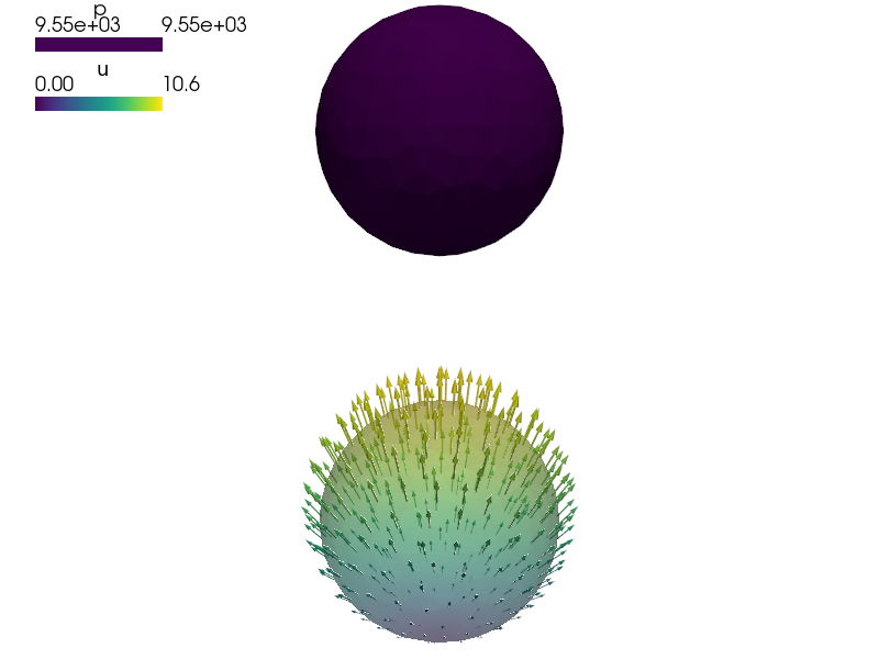
View the results using:
sfepy-view unit_ball.h5 -f u:wu:s12:p0 p:s12:p1
This example uses the adaptive time-stepping solver ('ts.adaptive') with
the default adaptivity function adapt_time_step(). Plot the used time steps by:
python3 sfepy/scripts/plot_times.py unit_ball.h5
r"""
Inflation of a Mooney-Rivlin hyperelastic balloon.
This example serves as a verification of the membrane term (``dw_tl_membrane``,
:class:`TLMembraneTerm <sfepy.terms.terms_membrane.TLMembraneTerm>`)
implementation.
Following Rivlin 1952 and Dumais, the analytical relation between a
relative stretch :math:`L = r / r_0` of a thin (membrane) sphere made of the
Mooney-Rivlin material of the undeformed radius :math:`r_0`, membrane
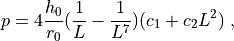
thickness :math:`h_0` and the inner pressure :math:`p` is
.. math::
p = 4 \frac{h_0}{r_0} (\frac{1}{L} - \frac{1}{L^7}) (c_1 + c_2 L^2) \;,
where :math:`c_1`, :math:`c_2` are the Mooney-Rivlin material parameters.
In the equations below, only the surface of the domain is mechanically
important - a stiff 2D membrane is embedded in the 3D space and coincides with
the balloon surface. The volume is very soft, to simulate a fluid-filled
cavity. A similar model could be used to model e.g. plant cells. The balloon
surface is loaded by prescribing the inner volume change :math:`\omega(t)`.
The fluid pressure in the cavity is a single scalar value, enforced either by
the ``'integral_mean_value'`` linear combination condition, when ``use_lcbcs``
argument of :func:`define()` is set to ``True`` (default), or by the
:math:`L^2` constant approximation.
Find :math:`\ul{u}(\ul{X})` and a constant :math:`p` such that:
- balance of forces:
.. math::
\intl{\Omega\suz}{} \left( \ull{S}\eff(\ul{u})
- p\; J \ull{C}^{-1} \right) : \delta \ull{E}(\ul{v}; \ul{v}) \difd{V}
+ \intl{\Gamma\suz}{} \ull{S}\eff(\tilde{\ul{u}}) \delta
\ull{E}(\tilde{\ul{u}}; \tilde{\ul{v}}) h_0 \difd{S}
= 0 \;, \quad \forall \ul{v} \in [H^1_0(\Omega)]^3 \;,
- volume conservation:
.. math::
\int\limits_{\Omega_0} \left[\omega(t)-J(u)\right] q\, dx = 0
\qquad \forall q \in L^2(\Omega) \;,
where
.. list-table::
:widths: 20 80
* - :math:`\ull{F}`
- deformation gradient :math:`F_{ij} = \pdiff{x_i}{X_j}`
* - :math:`J`
- :math:`\det(F)`
* - :math:`\ull{C}`
- right Cauchy-Green deformation tensor :math:`C = F^T F`
* - :math:`\ull{E}(\ul{u})`
- Green strain tensor :math:`E_{ij} = \frac{1}{2}(\pdiff{u_i}{X_j} +
\pdiff{u_j}{X_i} + \pdiff{u_m}{X_i}\pdiff{u_m}{X_j})`
* - :math:`\ull{S}\eff(\ul{u})`
- effective second Piola-Kirchhoff stress tensor
The effective stress :math:`\ull{S}\eff(\ul{u})` is given by:
.. math::
\ull{S}\eff(\ul{u}) = \mu J^{-\frac{2}{3}}(\ull{I}
- \frac{1}{3}\tr(\ull{C}) \ull{C}^{-1})
+ \kappa J^{-\frac{4}{3}} (\tr(\ull{C}\ull{I} - \ull{C}
- \frac{2}{6}((\tr{\ull{C}})^2 - \tr{(\ull{C}^2)})\ull{C}^{-1})
\;.
The :math:`\tilde{\ul{u}}` and :math:`\tilde{\ul{v}}` variables correspond to
:math:`\ul{u}`, :math:`\ul{v}`, respectively, transformed to the membrane
coordinate frame.
Use the following command to show a comparison of the FEM solution with the
above analytical relation (notice the nonlinearity of the dependence)::
sfepy-run sfepy/examples/large_deformation/balloon.py -d 'plot=True'
or::
sfepy-run sfepy/examples/large_deformation/balloon.py -d 'plot=True, use_lcbcs=False'
The agreement should be very good, even though the mesh is coarse.
View the results using::
sfepy-view unit_ball.h5 -f u:wu:s12:p0 p:s12:p1
This example uses the adaptive time-stepping solver (``'ts.adaptive'``) with
the default adaptivity function :func:`adapt_time_step()
<sfepy.solvers.ts_solvers.adapt_time_step>`. Plot the used time steps by::
python3 sfepy/scripts/plot_times.py unit_ball.h5
"""
import os
import numpy as nm
from sfepy.base.base import Output
from sfepy.discrete.fem import MeshIO
from sfepy.linalg import get_coors_in_ball
from sfepy import data_dir
output = Output('balloon:')
def get_nodes(coors, radius, eps, mode):
if mode == 'ax1':
centre = nm.array([0.0, 0.0, -radius], dtype=nm.float64)
elif mode == 'ax2':
centre = nm.array([0.0, 0.0, radius], dtype=nm.float64)
elif mode == 'equator':
centre = nm.array([radius, 0.0, 0.0], dtype=nm.float64)
else:
raise ValueError('unknown mode %s!' % mode)
return get_coors_in_ball(coors, centre, eps)
def get_volume(ts, coors, region=None, **kwargs):
rs = 1.0 + 1.0 * ts.time
rv = get_rel_volume(rs)
output('relative stretch:', rs)
output('relative volume:', rv)
out = nm.empty((coors.shape[0],), dtype=nm.float64)
out.fill(rv)
return out
def get_rel_volume(rel_stretch):
"""
Get relative volume V/V0 from relative stretch r/r0 of a ball.
"""
return nm.power(rel_stretch, 3.0)
def get_rel_stretch(rel_volume):
"""
Get relative stretch r/r0 from relative volume V/V0 of a ball.
"""
return nm.power(rel_volume, 1.0/3.0)
def get_balloon_pressure(rel_stretch, h0, r0, c1, c2):
"""
Rivlin 1952 + Dumais:
P = 4*h0/r0 * (1/L-1/L^7).*(C1+L^2*C2)
"""
L = rel_stretch
p = 4.0 * h0 / r0 * (1.0/L - 1.0/L**7) * (c1 + c2 * L**2)
return p
def plot_radius(problem, state):
import matplotlib.pyplot as plt
from sfepy.postprocess.time_history import extract_time_history
if problem.conf.use_lcbcs:
ths, ts = extract_time_history('unit_ball.h5', 'p e 0')
p = ths['p'][0]
else:
# Vertex 0 is not used in any cell...
ths, ts = extract_time_history('unit_ball.h5', 'p n 1')
p = ths['p'][1]
L = 1.0 + ts.times[:p.shape[0]]
L2 = 1.0 + nm.linspace(ts.times[0], ts.times[-1], 1000)
p2 = get_balloon_pressure(L2, 1e-2, 1, 3e5, 3e4)
plt.rcParams['lines.linewidth'] = 3
plt.rcParams['font.size'] = 14
plt.plot(L2, p2, 'r', label='theory')
plt.plot(L, p, 'b*', ms=12, label='FEM')
plt.title('Mooney-Rivlin hyperelastic balloon inflation')
plt.xlabel(r'relative stretch $r/r_0$')
plt.ylabel(r'pressure $p$')
plt.legend(loc='best')
plt.tight_layout()
fig = plt.gcf()
fig.savefig('balloon_pressure_stretch.pdf')
plt.show()
def define(plot=False, use_lcbcs=True):
filename_mesh = data_dir + '/meshes/3d/unit_ball.mesh'
conf_dir = os.path.dirname(__file__)
io = MeshIO.any_from_filename(filename_mesh, prefix_dir=conf_dir)
bbox = io.read_bounding_box()
dd = bbox[1] - bbox[0]
radius = bbox[1, 0]
eps = 1e-8 * dd[0]
options = {
'nls' : 'newton',
'ls' : 'ls',
'ts' : 'ts',
'save_times' : 'all',
'output_dir' : '.',
'output_format' : 'h5',
}
if plot:
options['post_process_hook_final'] = plot_radius
fields = {
'displacement': (nm.float64, 3, 'Omega', 1),
}
if use_lcbcs:
fields['pressure'] = (nm.float64, 1, 'Omega', 0)
else:
fields['pressure'] = (nm.float64, 1, 'Omega', 0, 'L2', 'constant')
materials = {
'solid' : ({
'mu' : 50, # shear modulus of neoHookean term
'kappa' : 0.0, # shear modulus of Mooney-Rivlin term
},),
'walls' : ({
'mu' : 3e5, # shear modulus of neoHookean term
'kappa' : 3e4, # shear modulus of Mooney-Rivlin term
'h0' : 1e-2, # initial thickness of wall membrane
},),
}
variables = {
'u' : ('unknown field', 'displacement', 0),
'v' : ('test field', 'displacement', 'u'),
'p' : ('unknown field', 'pressure', 1),
'q' : ('test field', 'pressure', 'p'),
'omega' : ('parameter field', 'pressure', {'setter' : 'get_volume'}),
}
regions = {
'Omega' : 'all',
'Ax1' : ('vertices by get_ax1', 'vertex'),
'Ax2' : ('vertices by get_ax2', 'vertex'),
'Equator' : ('vertices by get_equator', 'vertex'),
'Surface' : ('vertices of surface', 'facet'),
}
ebcs = {
'fix1' : ('Ax1', {'u.all' : 0.0}),
'fix2' : ('Ax2', {'u.[0, 1]' : 0.0}),
'fix3' : ('Equator', {'u.1' : 0.0}),
}
if use_lcbcs:
lcbcs = {
'pressure' : ('Omega', {'p.all' : None},
None, 'integral_mean_value'),
}
equations = {
'balance'
: """dw_tl_he_neohook.2.Omega(solid.mu, v, u)
+ dw_tl_he_mooney_rivlin.2.Omega(solid.kappa, v, u)
+ dw_tl_membrane.2.Surface(walls.mu, walls.kappa, walls.h0, v, u)
+ dw_tl_bulk_pressure.2.Omega(v, u, p)
= 0""",
'volume'
: """dw_tl_volume.2.Omega(q, u)
= dw_dot.2.Omega(q, omega)""",
}
solvers = {
'ls' : ('ls.auto_direct', {
# This setting causes a new factorization in each Newton step
# without computing the digest.
'use_presolve' : False,
'use_mtx_digest' : False,
}),
'newton' : ('nls.newton', {
'i_max' : 8,
'eps_a' : 1e-4,
'eps_r' : 1e-8,
'macheps' : 1e-16,
# Do not check linear system solution accuracy in each step.
'lin_red' : None,
'ls_red' : 0.5,
'ls_red_warp': 0.1,
'ls_on' : 100.0,
'ls_min' : 1e-5,
'check' : 0,
'delta' : 1e-6,
'report_status' : True,
}),
'ts' : ('ts.adaptive', {
't0' : 0.0,
't1' : 5.0,
'dt' : None,
'n_step' : 11,
'dt_red_factor' : 0.8,
'dt_red_max' : 1e-3,
'dt_inc_factor' : 1.25,
'dt_inc_on_iter' : 4,
'dt_inc_wait' : 3,
'verbose' : 1,
'quasistatic' : True,
}),
}
functions = {
'get_ax1' : (lambda coors, domain:
get_nodes(coors, radius, eps, 'ax1'),),
'get_ax2' : (lambda coors, domain:
get_nodes(coors, radius, eps, 'ax2'),),
'get_equator' : (lambda coors, domain:
get_nodes(coors, radius, eps, 'equator'),),
'get_volume' : (get_volume,),
}
return locals()