diffusion/sinbc.py

Description

Laplace equation with Dirichlet boundary conditions given by a sine function and constants.

Find such that:

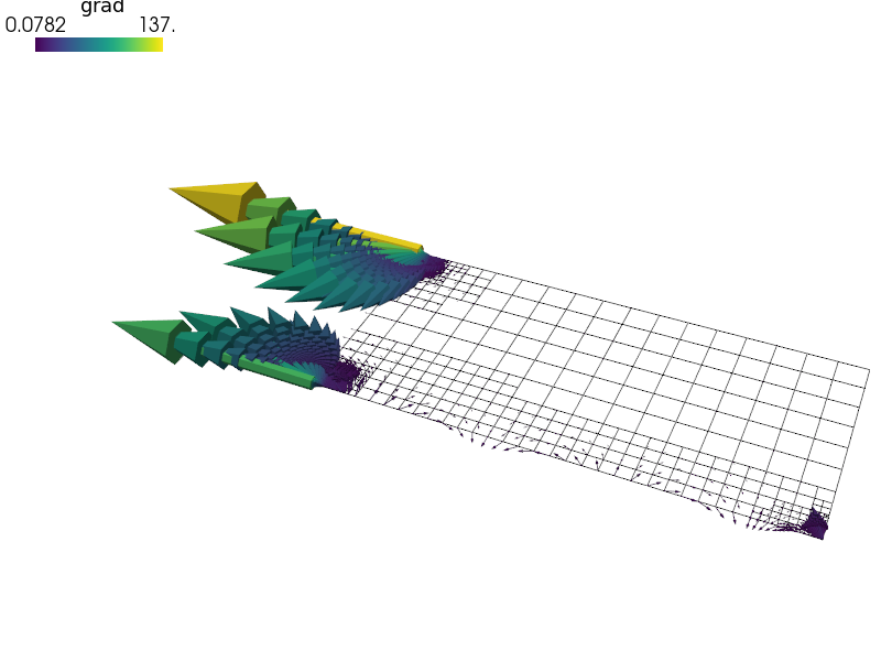
This example demonstrates how to use a hierarchical basis approximation - it uses the fifth order Lobatto polynomial space for the solution. The adaptive linearization is applied in order to save viewable results, see both the options keyword and the post_process() function that computes the solution gradient. Use the following commands to view the results (assuming default output directory and names):

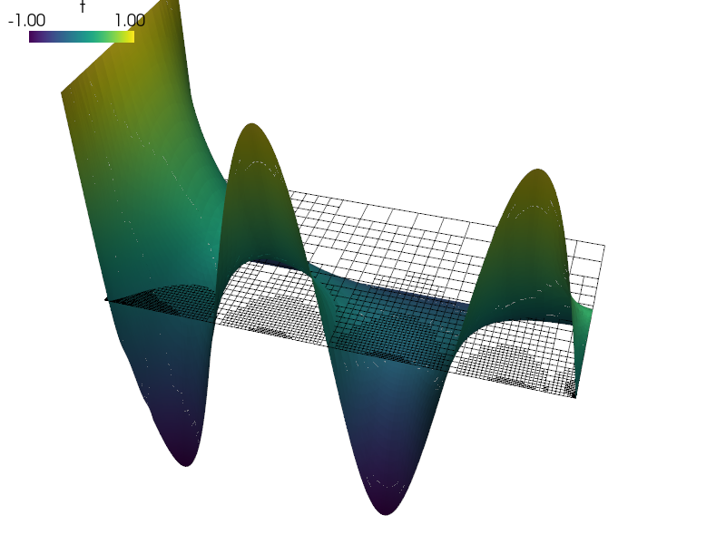
$ ./postproc.py -b -d't,plot_warp_scalar,rel_scaling=1' 2_4_2_refined_t.vtk --wireframe
$ ./postproc.py -b 2_4_2_refined_grad.vtk

The sfepy.discrete.fem.meshio.UserMeshIO class is used to refine the original two-element mesh before the actual solution.

source code

r"""
Laplace equation with Dirichlet boundary conditions given by a sine function
and constants.

Find :math:`t` such that:

.. math::
    \int_{\Omega} c \nabla s \cdot \nabla t
    = 0
    \;, \quad \forall s \;.

This example demonstrates how to use a hierarchical basis approximation - it
uses the fifth order Lobatto polynomial space for the solution. The adaptive
linearization is applied in order to save viewable results, see both the
options keyword and the ``post_process()`` function that computes the solution
gradient. Use the following commands to view the results (assuming default
output directory and names)::

  $ ./postproc.py -b -d't,plot_warp_scalar,rel_scaling=1' 2_4_2_refined_t.vtk --wireframe
  $ ./postproc.py -b 2_4_2_refined_grad.vtk

The :class:`sfepy.discrete.fem.meshio.UserMeshIO` class is used to refine the original
two-element mesh before the actual solution.
"""
from __future__ import absolute_import
import numpy as nm

from sfepy import data_dir

from sfepy.base.base import output
from sfepy.discrete.fem import Mesh, FEDomain
from sfepy.discrete.fem.meshio import UserMeshIO, MeshIO
from sfepy.homogenization.utils import define_box_regions
from six.moves import range

base_mesh = data_dir + '/meshes/elements/2_4_2.mesh'

def mesh_hook(mesh, mode):
    """
    Load and refine a mesh here.
    """
    if mode == 'read':
        mesh = Mesh.from_file(base_mesh)
        domain = FEDomain(mesh.name, mesh)
        for ii in range(3):
            output('refine %d...' % ii)
            domain = domain.refine()
            output('... %d nodes %d elements'
                   % (domain.shape.n_nod, domain.shape.n_el))

        domain.mesh.name = '2_4_2_refined'

        return domain.mesh

    elif mode == 'write':
        pass

def post_process(out, pb, state, extend=False):
    """
    Calculate gradient of the solution.
    """
    from sfepy.discrete.fem.fields_base import create_expression_output

    aux = create_expression_output('ev_grad.ie.Elements( t )',
                                   'grad', 'temperature',
                                   pb.fields, pb.get_materials(),
                                   pb.get_variables(), functions=pb.functions,
                                   mode='qp', verbose=False,
                                   min_level=0, max_level=5, eps=1e-3)
    out.update(aux)

    return out

filename_mesh = UserMeshIO(mesh_hook)

# Get the mesh bounding box.
io = MeshIO.any_from_filename(base_mesh)
bbox, dim = io.read_bounding_box(ret_dim=True)

options = {
    'nls' : 'newton',
    'ls' : 'ls',
    'post_process_hook' : 'post_process',
    'linearization' : {
        'kind' : 'adaptive',
        'min_level' : 0, # Min. refinement level to achieve everywhere.
        'max_level' : 5, # Max. refinement level.
        'eps' : 1e-3, # Relative error tolerance.
    },
}

materials = {
    'coef' : ({'val' : 1.0},),
}

regions = {
    'Omega' : 'all',
}
regions.update(define_box_regions(dim, bbox[0], bbox[1], 1e-5))

fields = {
    'temperature' : ('real', 1, 'Omega', 5, 'H1', 'lobatto'),
    # Compare with the Lagrange basis.
    ## 'temperature' : ('real', 1, 'Omega', 5, 'H1', 'lagrange'),
}

variables = {
    't' : ('unknown field', 'temperature', 0),
    's' : ('test field',    'temperature', 't'),
}

amplitude = 1.0
def ebc_sin(ts, coor, **kwargs):
    x0 = 0.5 * (coor[:, 1].min() + coor[:, 1].max())
    val = amplitude * nm.sin( (coor[:, 1] - x0) * 2. * nm.pi )
    return val

ebcs = {
    't1' : ('Left', {'t.0' : 'ebc_sin'}),
    't2' : ('Right', {'t.0' : -0.5}),
    't3' : ('Top', {'t.0' : 1.0}),
}

functions = {
    'ebc_sin' : (ebc_sin,),
}

equations = {
    'Temperature' : """dw_laplace.10.Omega( coef.val, s, t ) = 0"""
}

solvers = {
    'ls' : ('ls.scipy_direct', {}),
    'newton' : ('nls.newton', {
        'i_max'      : 1,
        'eps_a'      : 1e-10,
    }),
}