diffusion/poisson_periodic_boundary_condition.py
Description
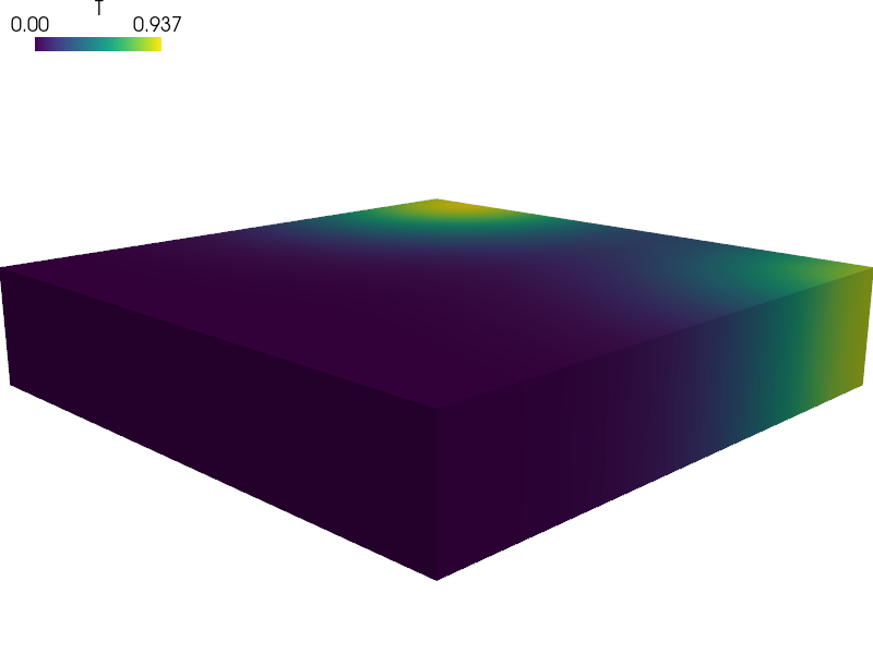
Transient Laplace equation with a localized power source and periodic boundary conditions.
This example is using a mesh generated by gmsh. Both the .geo script used by gmsh to generate the file and the .mesh file can be found in meshes.
The mesh is suitable for periodic boundary conditions. It consists of a cylinder enclosed by a box in the x and y directions.
The cylinder will act as a power source.
The transient Laplace equation will be solved in time interval
![t \in [0, t_{\rm final}]](../../_images/math/8c023166766d4c85ec4b41cd1ddee6f7040bffb9.png) .
.
Find  for such that:
r"""
Transient Laplace equation with a localized power source and
periodic boundary conditions.

This example is using a mesh generated by gmsh. Both the
.geo script used by gmsh to generate the file and the .mesh
file can be found in meshes.

The mesh is suitable for periodic boundary conditions. It consists
of a cylinder enclosed by a box in the x and y directions.

The cylinder will act as a power source.

The transient Laplace equation will be solved in time interval
:math:`t \in [0, t_{\rm final}]`.

Find :math:`T(t)` for :math:`t \in [0, t_{\rm final}]` such that:

.. math::
    \int_{\Omega}c s \pdiff{T}{t}
    + \int_{\Omega} \sigma_2 \nabla s \cdot \nabla T
    = \int_{\Omega_2} P_3 T
    \;, \quad \forall s \;.
"""

from __future__ import absolute_import
from sfepy import data_dir
import numpy as nm
import sfepy.discrete.fem.periodic as per

filename_mesh = data_dir + '/meshes/3d/cylinder_in_box.mesh'

t0 = 0.0
t1 = 1.
n_step = 11
power_per_volume =1.e2 # Heating power per volume of the cylinder
capacity_cylinder = 1. # Heat capacity of cylinder
capacity_fill = 1. #  Heat capacity of filling material
conductivity_cylinder = 1. # Heat conductivity of cylinder
conductivity_fill = 1. # Heat conductivity of filling material

def cylinder_material_func(ts, coors, problem, mode=None, **kwargs):
    """
    Returns the thermal conductivity, the thermal mass, and the power of the
    material in the cylinder.
    """
    if mode == 'qp':
        shape = (coors.shape[0], 1, 1)

        power = nm.empty(shape, dtype=nm.float64)
        if ts.step < 5:
            # The power is turned on in the first 5 steps only.
            power.fill(power_per_volume)

        else:
            power.fill(0.0)

        conductivity = nm.ones(shape) * conductivity_cylinder
        capacity = nm.ones(shape) * capacity_cylinder

        return {'power' : power, 'capacity' : capacity,
                'conductivity' : conductivity}

materials = {
    'cylinder' : 'cylinder_material_func',
    'fill' : ({'capacity' : capacity_fill,
               'conductivity' : conductivity_fill,},),
}

fields = {
    'temperature' : ('real', 1, 'Omega', 1),
}

variables = {
    'T' : ('unknown field', 'temperature', 1, 1),
    's' : ('test field', 'temperature', 'T'),
}

regions = {
    'Omega' : 'all',
    'cylinder' : 'cells of group 444',
    'fill' : 'cells of group 555',
    'Gamma_Left' : ('vertices in (x < -2.4999)', 'facet'),
    'y+' : ('vertices in (y >2.4999)', 'facet'),
    'y-' : ('vertices in (y <-2.4999)', 'facet'),
    'z+' : ('vertices in (z >0.4999)', 'facet'),
    'z-' : ('vertices in (z <-0.4999)', 'facet'),
}

ebcs = {
    'T1' : ('Gamma_Left', {'T.0' : 0.0}),
}

# The  matching functions link the elements on each side with that on the
# opposing side.
functions = {
    'cylinder_material_func' : (cylinder_material_func,),
    "match_y_plane" : (per.match_y_plane,),
    "match_z_plane" : (per.match_z_plane,),
}

epbcs = {
    # In the y-direction
    'periodic_y' : (['y+', 'y-'], {'T.0' : 'T.0'}, 'match_y_plane'),
    # and in the z-direction. Due to the symmetry of the problem, this periodic
    # boundary condition is actually not necessary, but we include it anyway.
    'periodic_z' : (['z+', 'z-'], {'T.0' : 'T.0'}, 'match_z_plane'),
}

ics = {
    'ic' : ('Omega', {'T.0' : 0.0}),
}

integrals = {
    'i' : 1,
}

equations = {
    'Temperature' :
    """dw_volume_dot.i.cylinder( cylinder.capacity, s, dT/dt )
        dw_volume_dot.i.fill( fill.capacity, s, dT/dt )
        dw_laplace.i.cylinder( cylinder.conductivity, s, T )
        dw_laplace.i.fill( fill.conductivity, s, T )
        = dw_volume_integrate.i.cylinder( cylinder.power, s )"""
}

solvers = {
    'ls' : ('ls.scipy_direct', {}),
    'newton' : ('nls.newton', {
        'i_max' : 1,
        'eps_a' : 1e-10,
        'eps_r' : 1.0,
    }),
    'ts' : ('ts.simple', {
        't0' : t0,
        't1' : t1,
        'dt' : None,
        'n_step' : n_step, # has precedence over dt!
        'quasistatic' : False,
        'verbose' : 1,
    }),
}

options = {
    'nls' : 'newton',
    'ls' : 'ls',
    'ts' : 'ts',
    'output_dir' : 'output',
    'save_times' : 'all',
    'active_only' : False,
}