acoustics/helmholtz_apartment.py

Description

A script demonstrating the solution of the scalar Helmholtz equation for a situation inspired by the physical problem of WiFi propagation in an apartment.

The example is an adaptation of the project found here: https://bthierry.pages.math.cnrs.fr/course-fem/projet/2017-2018/

The boundary conditions are defined as perfect radiation conditions, meaning that on the boundary waves will radiate outside.

The PDE for this physical process implies to find for such that:

Usage

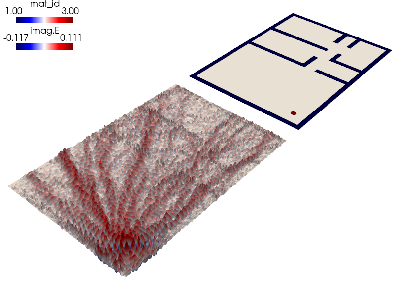
The mesh of the appartement and the different material ids can be visualized with the following:

sfepy-view meshes/2d/helmholtz_apartment.vtk -e -2

The example is run from the top level directory as:

sfepy-run sfepy/examples/acoustics/helmholtz_apartment.py

The result of the computation can be visualized as follows:

sfepy-view helmholtz_apartment.vtk --color-map=seismic -f imag.E:wimag.E:f10%:p0 --camera-position="-5.14968,-7.27948,7.08783,-0.463265,-0.23358,-0.350532,0.160127,0.664287,0.730124"

source code

r"""
A script demonstrating the solution of the scalar Helmholtz equation for a
situation inspired by the physical problem of WiFi propagation in an apartment.

The example is an adaptation of the project found here:
https://bthierry.pages.math.cnrs.fr/course-fem/projet/2017-2018/

The boundary conditions are defined as perfect radiation conditions, meaning
that on the boundary waves will radiate outside.

The PDE for this physical process implies to find :math:`E(x, t)` for :math:`x
\in \Omega` such that:

.. math::
    \left\lbrace
    \begin{aligned}
      \Delta E+ k^2 n(x)^2 E = f_s && \forall x \in \Omega \\
      \partial_n E(x)-ikn(x)E(x)=0 && \forall x \text{ on } \partial \Omega
    \end{aligned}
    \right.


Usage
-----

The mesh of the appartement and the different material ids can be visualized
with the following::

    sfepy-view meshes/2d/helmholtz_apartment.vtk -e -2

The example is run from the top level directory as::

    sfepy-run sfepy/examples/acoustics/helmholtz_apartment.py

The result of the computation can be visualized as follows::

    sfepy-view helmholtz_apartment.vtk --color-map=seismic -f imag.E:wimag.E:f10%:p0 --camera-position="-5.14968,-7.27948,7.08783,-0.463265,-0.23358,-0.350532,0.160127,0.664287,0.730124"
"""
import numpy as nm
from sfepy import data_dir

f = 2.4 * 1e9  # change this to 2.4 or 5 if you want to simulate frequencies
               # typically used by your Wifi
c0 = 3e8  # m/s
k = 2 * nm.pi * f / c0

filename_mesh = data_dir + "/meshes/2d/helmholtz_apartment.vtk"

regions = {
    'Omega': 'all',
    'Walls': ('cells of group 1'),
    'Air': ('cells of group 2'),
    'Source': ('cells of group 3'),
    'Gamma': ('vertices of surface', 'facet'),
}

# air and walls have different material parameters, hence the 1. and 2.4 factors
materials = {
    'material': ({'kn_square': {
        'Air': (k * 1.) ** 2,
        'Walls': (k * 2.4) ** 2}, },),
    'boundary': ({'kn': 1j * k * 2.4},),
    'source_func': 'source_func',
}


def source_func(ts, coors, mode=None, **kwargs):
    """The source function for the antenna."""
    epsilon = 0.1
    x_center = nm.array([-3.23, -1.58])
    if mode == 'qp':
        dists = nm.abs(nm.sum(nm.square(coors - x_center), axis=1))
        val = 3 / nm.pi / epsilon ** 2 * (1 - dists / epsilon)
        return {'val': val[:, nm.newaxis, nm.newaxis]}


functions = {
    'source_func': (source_func,),
}

fields = {
    'electric_field': ('complex', 1, 'Omega', 1),
}

variables = {
    'E': ('unknown field', 'electric_field', 1),
    'q': ('test field', 'electric_field', 'E'),
}

ebcs = {
}

integrals = {
    'i': 2,
}

equations = {
    'Helmholtz equation':
        """- dw_laplace.i.Omega(q, E)
        + dw_dot.i.Omega(material.kn_square, q, E)
        + dw_dot.i.Gamma(boundary.kn, q, E)
        = dw_integrate.i.Source(source_func.val, q)
        """
}

solvers = {
    'ls': ('ls.auto_direct', {}),
    'newton': ('nls.newton', {
        'i_max': 1,
    }),
}

options = {
    'refinement_level': 3,
}