multi_physics/thermo_elasticity_ess.py¶

Description

Thermo-elasticity with a computed temperature demonstrating equation sequence solver.

Uses dw_biot term with an isotropic coefficient for thermo-elastic coupling.

The equation sequence solver ('ess' in solvers) automatically solves first the temperature distribution and then the elasticity problem with the already computed temperature.

Find $\ul{u}$ , $T$ such that:

$\int_{\Omega} D_{ijkl}\ e_{ij}(\ul{v}) e_{kl}(\ul{u}) - \int_{\Omega} (T - T_0)\ \alpha_{ij} e_{ij}(\ul{v}) = 0 \;, \quad \forall \ul{v} \;, \int_{\Omega} \nabla s \cdot \nabla T = 0 \;, \quad \forall s \;.$

where

$D_{ijkl} = \mu (\delta_{ik} \delta_{jl}+\delta_{il} \delta_{jk}) + \lambda \ \delta_{ij} \delta_{kl} \;, \\ \alpha_{ij} = (3 \lambda + 2 \mu) \alpha \delta_{ij} \;,$

$T_0$ is the background temperature and $\alpha$ is the thermal expansion coefficient.

Notes¶

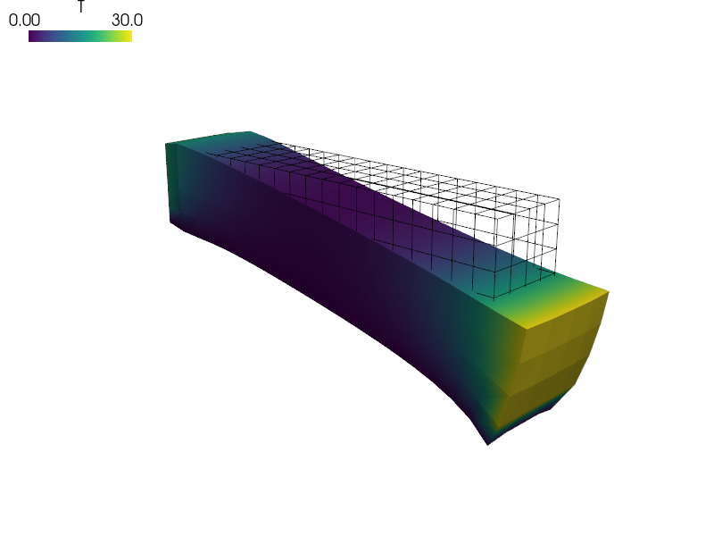
The gallery image was produced by (plus proper view settings):

sfepy-view block.vtk -f T:p1 u:wu:f1000:p0 u:vw:p0

../_images/multi_physics-thermo_elasticity_ess1.png

source code

r"""
Thermo-elasticity with a computed temperature demonstrating equation sequence
solver.

Uses `dw_biot` term with an isotropic coefficient for thermo-elastic coupling.

The equation sequence solver (``'ess'`` in ``solvers``) automatically solves
first the temperature distribution and then the elasticity problem with the
already computed temperature.

Find :math:`\ul{u}`, :math:`T` such that:

.. math::
    \int_{\Omega} D_{ijkl}\ e_{ij}(\ul{v}) e_{kl}(\ul{u})
    - \int_{\Omega}  (T - T_0)\ \alpha_{ij} e_{ij}(\ul{v})
    = 0
    \;, \quad \forall \ul{v} \;,

    \int_{\Omega} \nabla s \cdot \nabla T
    = 0
    \;, \quad \forall s \;.

where

.. math::
    D_{ijkl} = \mu (\delta_{ik} \delta_{jl}+\delta_{il} \delta_{jk}) +
    \lambda \ \delta_{ij} \delta_{kl}
    \;, \\

    \alpha_{ij} = (3 \lambda + 2 \mu) \alpha \delta_{ij} \;,

:math:`T_0` is the background temperature and :math:`\alpha` is the thermal
expansion coefficient.

Notes
-----
The gallery image was produced by (plus proper view settings)::

  sfepy-view block.vtk -f T:p1 u:wu:f1000:p0 u:vw:p0
"""
from __future__ import absolute_import
import numpy as np

from sfepy.mechanics.matcoefs import stiffness_from_lame
from sfepy import data_dir

# Material parameters.
lam = 10.0
mu = 5.0
thermal_expandability = 1.25e-5
T0 = 20.0 # Background temperature.

filename_mesh = data_dir + '/meshes/3d/block.mesh'

options = {
    'nls' : 'newton',
    'ls' : 'ls',

    'block_solve' : True,
}

regions = {
    'Omega' : 'all',
    'Left' : ('vertices in (x < -4.99)', 'facet'),
    'Right' : ('vertices in (x > 4.99)', 'facet'),
    'Bottom' : ('vertices in (z < -0.99)', 'facet'),
}

fields = {
    'displacement': ('real', 3, 'Omega', 1),
    'temperature': ('real', 1, 'Omega', 1),
}

variables = {
    'u' : ('unknown field', 'displacement', 0),
    'v' : ('test field', 'displacement', 'u'),
    'T' : ('unknown field', 'temperature', 1),
    's' : ('test field', 'temperature', 'T'),
}

ebcs = {
    'u0' : ('Left', {'u.all' : 0.0}),
    't0' : ('Left', {'T.0' : 20.0}),
    't2' : ('Bottom', {'T.0' : 0.0}),
    't1' : ('Right', {'T.0' : 30.0}),
}

eye_sym = np.array([[1], [1], [1], [0], [0], [0]], dtype=np.float64)
materials = {
    'solid' : ({
        'D' : stiffness_from_lame(3, lam=lam, mu=mu),
        'alpha' : (3.0 * lam + 2.0 * mu) * thermal_expandability * eye_sym
    },),
}

equations = {
    'balance_of_forces' : """
        + dw_lin_elastic.2.Omega(solid.D, v, u)
        - dw_biot.2.Omega(solid.alpha, v, T)
        = 0
    """,
    'temperature' : """
        + dw_laplace.1.Omega(s, T)
        = 0
    """
}

solvers = {
    'ls' : ('ls.scipy_direct', {}),
    'newton' : ('nls.newton', {
        'i_max'      : 1,
        'eps_a'      : 1e-10,
    }),
}