diffusion/sinbc.py
Description
Laplace equation with Dirichlet boundary conditions given by a sine function and constants.
Find  such that:
The sfepy.discrete.fem.meshio.UserMeshIO class is used to refine the
original two-element mesh before the actual solution.
The FE polynomial basis and the approximation order can be chosen on the
command-line. By default, the fifth order Lagrange polynomial space is used,
see define() arguments.
This example demonstrates how to visualize higher order approximations of the
continuous solution. The adaptive linearization is applied in order to save
viewable results, see both the options keyword and the post_process()
function that computes the solution gradient. The linearization parameters can
also be specified on the command line.
The Lagrange or Bernstein polynomial bases support higher order DOFs in the Dirichlet boundary conditions, unlike the hierarchical Lobatto basis implementation, compare the results of:
sfepy-run sfepy/examples/diffusion/sinbc.py -d basis=lagrange
sfepy-run sfepy/examples/diffusion/sinbc.py -d basis=bernstein
sfepy-run sfepy/examples/diffusion/sinbc.py -d basis=lobatto
Use the following commands to view each of the results of the above commands (assuming default output directory and names):
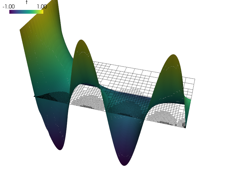
sfepy-view 2_4_2_refined_t.vtk -2 -f t:wt
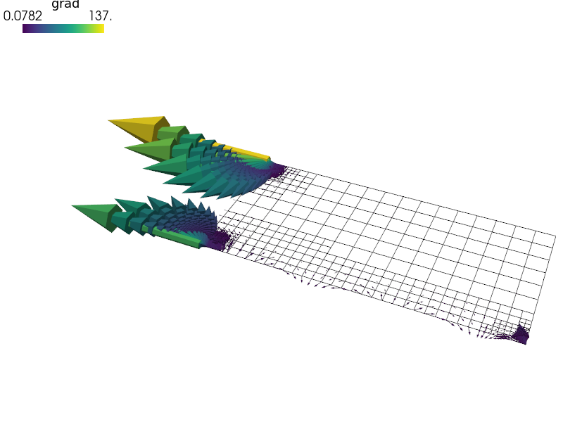
sfepy-view 2_4_2_refined_grad.vtk -2
r"""
Laplace equation with Dirichlet boundary conditions given by a sine function
and constants.

Find :math:`t` such that:

.. math::
    \int_{\Omega} c \nabla s \cdot \nabla t
    = 0
    \;, \quad \forall s \;.

The :class:`sfepy.discrete.fem.meshio.UserMeshIO` class is used to refine the
original two-element mesh before the actual solution.

The FE polynomial basis and the approximation order can be chosen on the
command-line. By default, the fifth order Lagrange polynomial space is used,
see ``define()`` arguments.

This example demonstrates how to visualize higher order approximations of the
continuous solution. The adaptive linearization is applied in order to save
viewable results, see both the options keyword and the ``post_process()``
function that computes the solution gradient. The linearization parameters can
also be specified on the command line.

The Lagrange or Bernstein polynomial bases support higher order
DOFs in the Dirichlet boundary conditions, unlike the hierarchical Lobatto
basis implementation, compare the results of::

  sfepy-run sfepy/examples/diffusion/sinbc.py -d basis=lagrange
  sfepy-run sfepy/examples/diffusion/sinbc.py -d basis=bernstein
  sfepy-run sfepy/examples/diffusion/sinbc.py -d basis=lobatto

Use the following commands to view each of the results of the above commands
(assuming default output directory and names)::

  sfepy-view 2_4_2_refined_t.vtk -2 -f t:wt
  sfepy-view 2_4_2_refined_grad.vtk -2
"""
import numpy as nm

from sfepy import data_dir

from sfepy.base.base import output
from sfepy.discrete.fem import Mesh, FEDomain
from sfepy.discrete.fem.meshio import UserMeshIO, MeshIO
from sfepy.homogenization.utils import define_box_regions

base_mesh = data_dir + '/meshes/elements/2_4_2.mesh'

def mesh_hook(mesh, mode):
    """
    Load and refine a mesh here.
    """
    if mode == 'read':
        mesh = Mesh.from_file(base_mesh)
        domain = FEDomain(mesh.name, mesh)
        for ii in range(3):
            output('refine %d...' % ii)
            domain = domain.refine()
            output('... %d nodes %d elements'
                   % (domain.shape.n_nod, domain.shape.n_el))

        domain.mesh.name = '2_4_2_refined'

        return domain.mesh

    elif mode == 'write':
        pass

def post_process(out, pb, state, extend=False):
    """
    Calculate gradient of the solution.
    """
    from sfepy.discrete.fem.fields_base import create_expression_output

    aux = create_expression_output('ev_grad.ie.Elements( t )',
                                   'grad', 'temperature',
                                   pb.fields, pb.get_materials(),
                                   pb.get_variables(), functions=pb.functions,
                                   mode='qp', verbose=False,
                                   min_level=0, max_level=5, eps=1e-3)
    out.update(aux)

    return out

def define(order=5, basis='lagrange', min_level=0, max_level=5, eps=1e-3):

    filename_mesh = UserMeshIO(mesh_hook)

    # Get the mesh bounding box.
    io = MeshIO.any_from_filename(base_mesh)
    bbox, dim = io.read_bounding_box(ret_dim=True)

    options = {
        'nls' : 'newton',
        'ls' : 'ls',
        'post_process_hook' : 'post_process',
        'linearization' : {
            'kind' : 'adaptive',
            'min_level' : min_level, # Min. refinement level applied everywhere.
            'max_level' : max_level, # Max. refinement level.
            'eps' : eps, # Relative error tolerance.
        },
    }

    materials = {
        'coef' : ({'val' : 1.0},),
    }

    regions = {
        'Omega' : 'all',
    }
    regions.update(define_box_regions(dim, bbox[0], bbox[1], 1e-5))

    fields = {
        'temperature' : ('real', 1, 'Omega', order, 'H1', basis),
    }

    variables = {
        't' : ('unknown field', 'temperature', 0),
        's' : ('test field',    'temperature', 't'),
    }

    amplitude = 1.0
    def ebc_sin(ts, coor, **kwargs):
        x0 = 0.5 * (coor[:, 1].min() + coor[:, 1].max())
        val = amplitude * nm.sin( (coor[:, 1] - x0) * 2. * nm.pi )
        return val

    ebcs = {
        't1' : ('Left', {'t.0' : 'ebc_sin'}),
        't2' : ('Right', {'t.0' : -0.5}),
        't3' : ('Top', {'t.0' : 1.0}),
    }

    functions = {
        'ebc_sin' : (ebc_sin,),
    }

    equations = {
        'Temperature' : """dw_laplace.10.Omega(coef.val, s, t) = 0"""
    }

    solvers = {
        'ls' : ('ls.scipy_direct', {}),
        'newton' : ('nls.newton', {
            'i_max'      : 1,
            'eps_a'      : 1e-10,
        }),
    }

    return locals()