Mesh parametrization
Introduction
When dealing with shape optimization we usually need to modify a FE mesh using a few optimization parameters describing the mesh geometry. The B-spline parametrization offers an efficient way to do that. A mesh region (2D or 3D) that is to be parametrized is enclosed in the so called spline-box and the positions of all vertices inside the box can be changed by moving the control points of the B-spline curves.
There are two different classes for the B-spline parametrization implemented in
SfePy (module sfepy.mesh.splinebox): SplineBox and
SplineRegion2D. The first one defines a rectangular parametrization box in
2D or 3D while the second one allows to set up an arbitrary shaped region of
parametrization in 2D.
SplineBox
The rectangular B-spline parametrization is created as follows:
1from sfepy.mesh.splinebox import SplineBox
2
3spb = SplineBox(<bbox>, <coors>, <nsg>)
the first parameter defines the range of the box in each dimension, the second
parameter is the array of coordinates (vertices) to be parametrized and the
last one (optional) determines the number of control points in each dimension.
The number of the control points ( ) is calculated as:
(1)
where  is the degree of the B-spline curve (default value: 3 =
cubic spline) and
is the degree of the B-spline curve (default value: 3 =
cubic spline) and  is the number of the spline segments (default
value: [1,1(,1)] = 4 control points for all dimensions).
is the number of the spline segments (default
value: [1,1(,1)] = 4 control points for all dimensions).
The position of the vertices can be modified by moving the control points:
spb.move_control_point(<cpoint>, <val>)
where <cpoint> is the index or position of the control point, for explanation see the following figure.
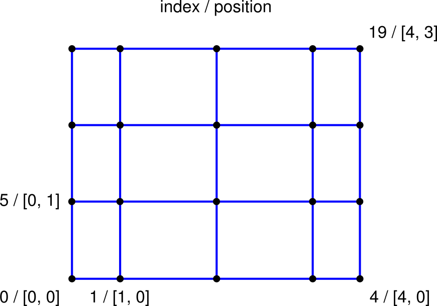
The displacement is given by <val>. The modified coordinates of the vertices are evaluated by:
new_coors = spb.evaluate()
Example
Create a new 2D
SplineBoxwith the left bottom corner at [-1,-1] and the right top corner at [1, 0.6] which has 5 control points in x-direction and 4 control points in y-direction:1from sfepy.mesh.splinebox import SplineBox 2from sfepy.discrete.fem import Mesh 3 4mesh = Mesh.from_file('meshes/2d/square_tri1.mesh') 5spb = SplineBox([[-1, 1], [-1, 0.6]], mesh.coors, nsg=[2,1])
Modify the position of mesh coordinates by moving three control points (with indices 1,2 and 3):
1spb.move_control_point(1, [0.1, -0.2])
2spb.move_control_point(2, [0.2, -0.3])
3spb.move_control_point(3, [0.0, -0.1])
Evaluate the new coordinates:
mesh.cmesh.coors[:] = spb.evaluate()
Write the deformed mesh and the spline control net (the net of control points) into vtk files:
spb.write_control_net('square_tri1_spbox.vtk')
mesh.write('square_tri1_deform.vtk')
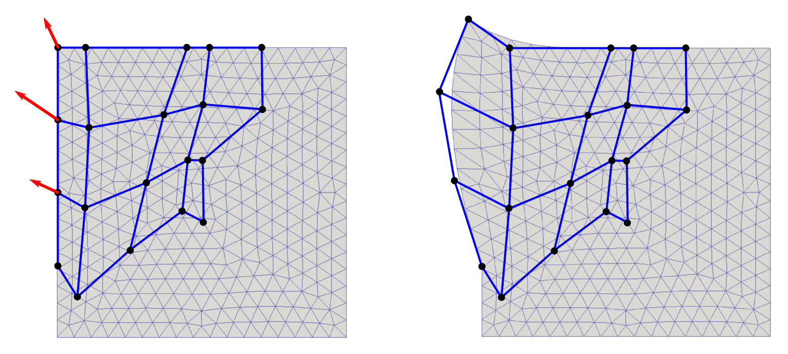
The following figures show the undeformed (left) and deformed (right) mesh and the control net.
SplineRegion2D
In this case, the region (only in 2D) of parametrization is defined by four B-spline curves:
1from sfepy.mesh.splinebox import SplineRegion2D
2
3spb = SplineRegion2D([<bspl1>, <bspl2>, <bspl3>, <bspl4>], <coors>)
The curves must form a closed loop, must be oriented counterclockwise and the opposite curves (<bspl1>, <bspl3> and <bspl2>, <bspl4>) must have the same number of control points and the same knot vectors, see the figure below, on the left.
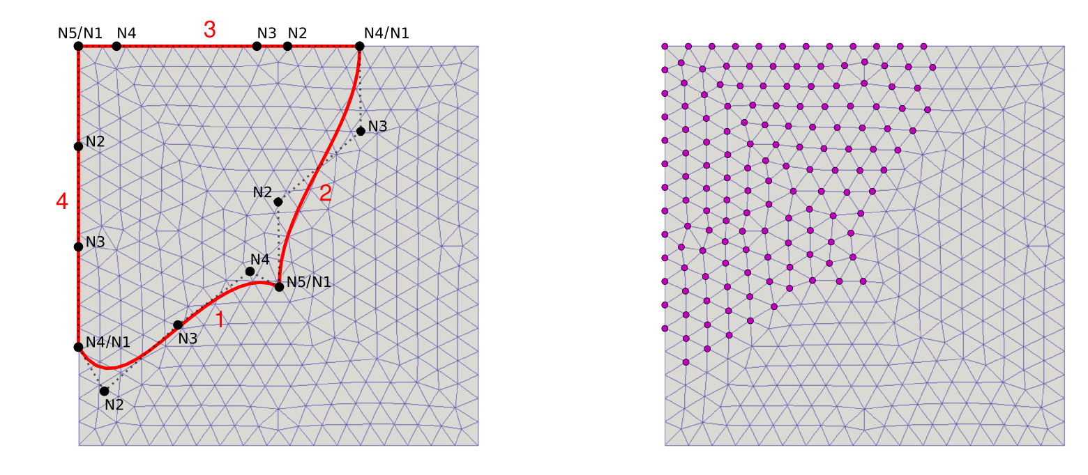
The position of the selected vertices, depicted in the figure on the right, are
driven by the control points in the same way as explained above for
SplineBox.
Note: Initializing SplineRegion2D may be time consuming due to the fact
that for all vertex coordinates the spline parameters have to be found using
an optimization method in which the B-spline basis is repeatedly evaluated.
Example
First of all, define four B-spline curves (the default degree of the spline curve is 3) representing the boundary of a parametrization area:
 1from sfepy.mesh.bspline import BSpline
 2
 3# left / right boundary
 4line_l = nm.array([[-1, 1], [-1, .5], [-1, 0], [-1, -.5]])
 5line_r = nm.array([[0, -.2], [.1, .2], [.3, .6], [.4, 1]])
 6
 7sp_l = BSpline()
 8sp_l.approximate(line_l, ncp=4)
 9kn_lr = sp_l.get_knot_vector()
10
11sp_r = BSpline()
12sp_r.approximate(line_r, knots=kn_lr)
13
14# bottom / top boundary
15line_b = nm.array([[-1, -.5], [-.8, -.6], [-.5, -.4], [-.2, -.2], [0, -.2]])
16line_t = nm.array([[.4, 1], [0, 1], [-.2, 1], [-.6, 1], [-1, 1]])
17
18sp_b = BSpline()
19sp_b.approximate(line_b, ncp=5)
20kn_bt = sp_b.get_knot_vector()
21
22sp_t = BSpline()
23sp_t.approximate(line_t, knots=kn_bt)
Create a new 2D
SplineRegion2Dobject:1from sfepy.mesh.splinebox import SplineRegion2D 2 3spb = SplineRegion2D([sp_b, sp_r, sp_t, sp_l], mesh.coors)
Move the control points:
1spb.move_control_point(5, [-.2, .1])
2spb.move_control_point(10, [-.3, .2])
3spb.move_control_point(15, [-.1, .2])
Evaluate the new coordinates:
mesh.cmesh.coors[:] = spb.evaluate()
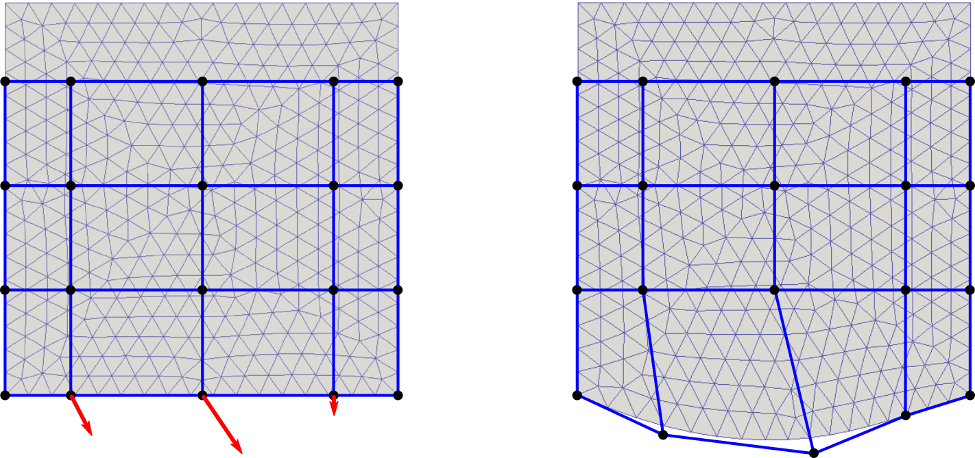
The figures below show the undeformed (left) and deformed (right) mesh and the control net.