linear_elasticity/elastic2D_axisymmetric.py¶

Description

Axisymmetric Linear Elasticity (2D formulation).

This example demonstrates a two-dimensional axisymmetric formulation of the three-dimensional static linear elasticity equations. The formulation is derived under the standard axisymmetry assumptions and is equivalent to the original three-dimensional problem.

Three-dimensional linear elasticity¶

Let $\Omega_{3D} \subset \mathbb{R}^3$ denote an elastic body. The static equilibrium equations read

$\nabla \cdot \boldsymbol{\sigma} + \boldsymbol{b} = 0 \quad \text{in } \Omega_{3D}.$

In the absence of body forces ( $\boldsymbol{b} = 0$ ),

$\nabla \cdot \boldsymbol{\sigma} = 0.$

The material is assumed to be linear, isotropic, and homogeneous, with the constitutive relation

$\boldsymbol{\sigma} = 2\mu\,\boldsymbol{\varepsilon}(\boldsymbol{u}) + \lambda\,\mathrm{tr} \bigl(\boldsymbol{\varepsilon}(\boldsymbol{u})\bigr)\mathbf{I},$

where the infinitesimal strain tensor is defined as

$\boldsymbol{\varepsilon}(\boldsymbol{u}) = \frac{1}{2}\bigl( \nabla\boldsymbol{u} + (\nabla\boldsymbol{u})^{T} \bigr).$

Axisymmetric assumptions¶

Cylindrical coordinates $(r, \theta, z)$ are introduced. The following assumptions are made:

all fields are independent of $\theta$ ,
the circumferential displacement vanishes: $u_\theta = 0$ .

The displacement field therefore reduces to

$\boldsymbol{u}(r, z) = (u_r(r, z),\, 0,\, u_z(r, z)).$

The computational domain is the meridian cross-section

$\Omega \subset \mathbb{R}^2_{(r, z)}.$

Axisymmetric strong form¶

Radial equilibrium¶

$\partial_r \sigma_{rr} + \partial_z \sigma_{rz} + \frac{\sigma_{rr} - \sigma_{\theta\theta}}{r} = 0 \quad \text{in } \Omega.$

Axial equilibrium¶

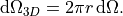
$\partial_r \sigma_{rz} + \partial_z \sigma_{zz} + \frac{\sigma_{rz}}{r} = 0 \quad \text{in } \Omega.$

Axisymmetric weak formulation¶

Let $v_r$ and $v_z$ denote admissible test functions. Assuming zero traction boundary conditions, integration over the circumferential direction yields the axisymmetric volume element

$\mathrm{d}\Omega_{3D} = 2\pi r\,\mathrm{d}\Omega.$

Radial equilibrium (weak form)¶

$\int_\Omega \bigl( \sigma_{rr}\,\partial_r v_r + \sigma_{rz}\,\partial_z v_r \bigr)(2\pi r)\,\mathrm{d}\Omega + \int_\Omega \sigma_{\theta\theta}\,v_r\,(2\pi)\,\mathrm{d}\Omega = 0.$

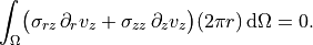
Axial equilibrium (weak form)¶

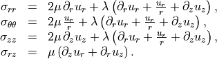
$\int_\Omega \bigl( \sigma_{rz}\,\partial_r v_z + \sigma_{zz}\,\partial_z v_z \bigr)(2\pi r)\,\mathrm{d}\Omega = 0.$

Stress–strain relations in axisymmetry¶

The nonzero stress components in axisymmetry are

$\begin{array}{rcl} \sigma_{rr} &=& 2\mu\,\partial_r u_r + \lambda\left(\partial_r u_r + \frac{u_r}{r} + \partial_z u_z\right), \\ \sigma_{\theta\theta} &=& 2\mu\,\frac{u_r}{r} + \lambda\left(\partial_r u_r + \frac{u_r}{r} + \partial_z u_z\right), \\ \sigma_{zz} &=& 2\mu\,\partial_z u_z + \lambda\left(\partial_r u_r + \frac{u_r}{r} + \partial_z u_z\right), \\ \sigma_{rz} &=& \mu\left(\partial_z u_r + \partial_r u_z\right). \end{array}$

Compact bilinear form¶

Radial test function¶

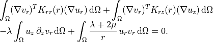
$\begin{array}{l} \displaystyle \int_{\Omega} (\nabla v_r)^{T} K_{rr}(r) (\nabla u_r)\,\mathrm{d}\Omega + \int_{\Omega} (\nabla v_r)^{T} K_{rz}(r) (\nabla u_z)\,\mathrm{d}\Omega \\ \displaystyle - \lambda \int_{\Omega} u_z\,\partial_z v_r\,\mathrm{d}\Omega + \int_{\Omega} \frac{\lambda + 2\mu}{r}\, u_r v_r\,\mathrm{d}\Omega = 0. \end{array}$

Axial test function¶

$\begin{array}{l} \displaystyle \int_{\Omega} (\nabla v_z)^{T} K_{zr}(r) (\nabla u_r)\,\mathrm{d}\Omega + \int_{\Omega} (\nabla v_z)^{T} K_{zz}(r) (\nabla u_z)\,\mathrm{d}\Omega\\ \displaystyle + \lambda \int_{\Omega} u_r\,\partial_z v_z\,\mathrm{d}\Omega = 0. \end{array}$

Axisymmetric material matrices¶

$K_{rr}(r) = r \left[ \begin{array}{cc} \lambda + 2\mu & 0 \\ 0 & \mu \end{array} \right], \qquad K_{rz}(r) = r \left[ \begin{array}{cc} 0 & \lambda \\ \mu & 0 \end{array} \right].$

$K_{zr}(r) = r \left[ \begin{array}{cc} 0 & \mu \\ \lambda & 0 \end{array} \right], \qquad K_{zz}(r) = r \left[ \begin{array}{cc} \mu & 0 \\ 0 & \lambda + 2\mu \end{array} \right].$

Remark¶

This formulation is mathematically equivalent to the original three-dimensional linear elasticity problem under the stated axisymmetry assumptions. It is directly suitable for two-dimensional finite element discretizations using the axisymmetric weighting.

To run the example, execute one of the following commands:

python3 -m sfepy.scripts.simple ./sfepy/examples/linear_elasticity/elastic2D_axisymmetric.py
sfepy-run sfepy/examples/linear_elasticity/elastic2D_axisymmetric.py

../_images/linear_elasticity-elastic2D_axisymmetric.png

source code

r"""
Axisymmetric Linear Elasticity (2D formulation).

This example demonstrates a two-dimensional axisymmetric formulation of the
three-dimensional static linear elasticity equations. The formulation is derived
under the standard axisymmetry assumptions and is equivalent to the original
three-dimensional problem.

Three-dimensional linear elasticity
-----------------------------------

Let :math:`\Omega_{3D} \subset \mathbb{R}^3` denote an elastic body. The static
equilibrium equations read

.. math::
   \nabla \cdot \boldsymbol{\sigma} + \boldsymbol{b} = 0
   \quad \text{in } \Omega_{3D}.

In the absence of body forces (:math:`\boldsymbol{b} = 0`),

.. math::
   \nabla \cdot \boldsymbol{\sigma} = 0.

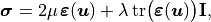
The material is assumed to be linear, isotropic, and homogeneous, with the
constitutive relation

.. math::
   \boldsymbol{\sigma}
   = 2\mu\,\boldsymbol{\varepsilon}(\boldsymbol{u})
   + \lambda\,\mathrm{tr}
     \bigl(\boldsymbol{\varepsilon}(\boldsymbol{u})\bigr)\mathbf{I},

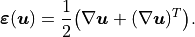
where the infinitesimal strain tensor is defined as

.. math::
   \boldsymbol{\varepsilon}(\boldsymbol{u})
   = \frac{1}{2}\bigl(
     \nabla\boldsymbol{u} + (\nabla\boldsymbol{u})^{T}
     \bigr).

Axisymmetric assumptions
------------------------

Cylindrical coordinates :math:`(r, \theta, z)` are introduced. The following
assumptions are made:

- all fields are independent of :math:`\theta`,
- the circumferential displacement vanishes: :math:`u_\theta = 0`.

The displacement field therefore reduces to

.. math::
   \boldsymbol{u}(r, z) = (u_r(r, z),\, 0,\, u_z(r, z)).

The computational domain is the meridian cross-section

.. math::
   \Omega \subset \mathbb{R}^2_{(r, z)}.

Axisymmetric strong form
------------------------

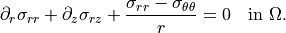
Radial equilibrium
~~~~~~~~~~~~~~~~~~

.. math::
   \partial_r \sigma_{rr}
   + \partial_z \sigma_{rz}
   + \frac{\sigma_{rr} - \sigma_{\theta\theta}}{r}
   = 0
   \quad \text{in } \Omega.

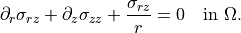
Axial equilibrium
~~~~~~~~~~~~~~~~~

.. math::
   \partial_r \sigma_{rz}
   + \partial_z \sigma_{zz}
   + \frac{\sigma_{rz}}{r}
   = 0
   \quad \text{in } \Omega.

Axisymmetric weak formulation
-----------------------------

Let :math:`v_r` and :math:`v_z` denote admissible test functions. Assuming zero
traction boundary conditions, integration over the circumferential direction
yields the axisymmetric volume element

.. math::
   \mathrm{d}\Omega_{3D} = 2\pi r\,\mathrm{d}\Omega.

Radial equilibrium (weak form)
~~~~~~~~~~~~~~~~~~~~~~~~~~~~~~

.. math::
   \int_\Omega
   \bigl(
     \sigma_{rr}\,\partial_r v_r
     + \sigma_{rz}\,\partial_z v_r
   \bigr)(2\pi r)\,\mathrm{d}\Omega
   + \int_\Omega
     \sigma_{\theta\theta}\,v_r\,(2\pi)\,\mathrm{d}\Omega
   = 0.

Axial equilibrium (weak form)
~~~~~~~~~~~~~~~~~~~~~~~~~~~~~

.. math::
   \int_\Omega
   \bigl(
     \sigma_{rz}\,\partial_r v_z
     + \sigma_{zz}\,\partial_z v_z
   \bigr)(2\pi r)\,\mathrm{d}\Omega
   = 0.

Stress--strain relations in axisymmetry
---------------------------------------

The nonzero stress components in axisymmetry are

.. math::

   \begin{array}{rcl}
   \sigma_{rr} &=&
   2\mu\,\partial_r u_r
   + \lambda\left(\partial_r u_r + \frac{u_r}{r} + \partial_z u_z\right), \\
   \sigma_{\theta\theta} &=&
   2\mu\,\frac{u_r}{r}
   + \lambda\left(\partial_r u_r + \frac{u_r}{r} + \partial_z u_z\right), \\
   \sigma_{zz} &=&
   2\mu\,\partial_z u_z
   + \lambda\left(\partial_r u_r + \frac{u_r}{r} + \partial_z u_z\right), \\
   \sigma_{rz} &=&
   \mu\left(\partial_z u_r + \partial_r u_z\right).
   \end{array}


Compact bilinear form
---------------------

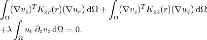
Radial test function
~~~~~~~~~~~~~~~~~~~~

.. math::

   \begin{array}{l}
   \displaystyle
   \int_{\Omega} (\nabla v_r)^{T} K_{rr}(r) (\nabla u_r)\,\mathrm{d}\Omega
   + \int_{\Omega} (\nabla v_r)^{T} K_{rz}(r) (\nabla u_z)\,\mathrm{d}\Omega \\
   \displaystyle
   - \lambda \int_{\Omega} u_z\,\partial_z v_r\,\mathrm{d}\Omega
   + \int_{\Omega} \frac{\lambda + 2\mu}{r}\, u_r v_r\,\mathrm{d}\Omega
   = 0.
   \end{array}

Axial test function
~~~~~~~~~~~~~~~~~~~

.. math::

   \begin{array}{l}
   \displaystyle
   \int_{\Omega} (\nabla v_z)^{T} K_{zr}(r) (\nabla u_r)\,\mathrm{d}\Omega
   + \int_{\Omega} (\nabla v_z)^{T} K_{zz}(r) (\nabla u_z)\,\mathrm{d}\Omega\\
   \displaystyle
   + \lambda \int_{\Omega} u_r\,\partial_z v_z\,\mathrm{d}\Omega
   = 0.
   \end{array}

Axisymmetric material matrices
------------------------------

.. math::

   K_{rr}(r) = r
   \left[
   \begin{array}{cc}
   \lambda + 2\mu & 0 \\
   0 & \mu
   \end{array}
   \right],
   \qquad
   K_{rz}(r) = r
   \left[
   \begin{array}{cc}
   0 & \lambda \\
   \mu & 0
   \end{array}
   \right].

.. math::

   K_{zr}(r) = r
   \left[
   \begin{array}{cc}
   0 & \mu \\
   \lambda & 0
   \end{array}
   \right],
   \qquad
   K_{zz}(r) = r
   \left[
   \begin{array}{cc}
   \mu & 0 \\
   0 & \lambda + 2\mu
   \end{array}
   \right].


Remark
------

This formulation is mathematically equivalent to the original three-dimensional
linear elasticity problem under the stated axisymmetry assumptions. It is
directly suitable for two-dimensional finite element discretizations using the
axisymmetric weighting.

To run the example, execute one of the following commands::

   python3 -m sfepy.scripts.simple ./sfepy/examples/linear_elasticity/elastic2D_axisymmetric.py
   sfepy-run sfepy/examples/linear_elasticity/elastic2D_axisymmetric.py
"""

import numpy as np

E = 70e9
nu = 0.3

r_inner, r_outer = 0.1, 0.2
height = 0.3

a, b = 1e-3, 2e-3


def define():
    from sfepy.discrete.fem import Mesh
    from sfepy.homogenization.utils import define_box_regions

    lam = E * nu / ((1 + nu) * (1 - 2 * nu))
    mu = E / (2 * (1 + nu))

    nr, nz = 9, 11
    r = np.linspace(r_inner, r_outer, nr)
    z = np.linspace(0.0, height, nz)

    nodes = []
    for iz in range(nz):
        for ir in range(nr):
            nodes.append([r[ir], z[iz]])
    coors = np.array(nodes, dtype=np.float64)

    conn = []
    for iz in range(nz - 1):
        for ir in range(nr - 1):
            n0 = iz * nr + ir
            conn.append([n0, n0 + 1, n0 + nr + 1, n0 + nr])
    conn = np.array(conn, dtype=np.int32)

    filename_mesh = mesh = Mesh.from_data(
        "annulus",
        coors,
        None,
        [conn],
        [np.zeros(len(conn), dtype=np.int32)],
        ["2_4"],
    )

    # Get bounding box for region definition
    bbox = mesh.get_bounding_box()

    # -----------------------------
    # Material coefficient functions
    # -----------------------------
    def material_rr(ts, coors, mode=None, **kwargs):
        if mode == "qp":
            rr = coors[:, 0]
            K = np.zeros((coors.shape[0], 2, 2), dtype=np.float64)
            K[:, 0, 0] = (lam + 2 * mu) * rr
            K[:, 1, 1] = mu * rr
            return {"K": K}

    def material_zz(ts, coors, mode=None, **kwargs):
        if mode == "qp":
            rr = coors[:, 0]
            K = np.zeros((coors.shape[0], 2, 2), dtype=np.float64)
            K[:, 0, 0] = mu * rr
            K[:, 1, 1] = (lam + 2 * mu) * rr
            return {"K": K}

    def material_poisson_rr(ts, coors, mode=None, **kwargs):
        if mode == "qp":
            rr = coors[:, 0]
            K = np.zeros((coors.shape[0], 2, 2), dtype=np.float64)
            K[:, 0, 1] = mu * rr
            K[:, 1, 0] = lam * rr
            return {"K": K}

    def material_poisson_zz(ts, coors, mode=None, **kwargs):
        if mode == "qp":
            rr = coors[:, 0]
            K = np.zeros((coors.shape[0], 2, 2), dtype=np.float64)
            K[:, 0, 1] = lam * rr
            K[:, 1, 0] = mu * rr
            return {"K": K}

    def material_hoop0(ts, coors, mode=None, **kwargs):
        if mode == "qp":
            rr = coors[:, 0]
            rr_safe = np.maximum(rr, 1e-12)
            c = (lam + 2 * mu) / rr_safe
            return {"c": c.reshape(-1, 1, 1)}

    # -----------------------------
    # Regions: Use define_box_regions for automatic boundary selection
    # -----------------------------
    regions = {
        "Omega": "all",
    }
    regions.update(define_box_regions(2, bbox[0], bbox[1]))

    materials = {
        "m_rr": "material_rr",
        "m_zz": "material_zz",
        "m_prr": "material_poisson_rr",
        "m_pzz": "material_poisson_zz",
        "m_hoop_idx": ({'.val' : np.array([[1]])},),
        "m_hoop0": "material_hoop0",
    }

    fields = {
        "ur": ("real", 1, "Omega", 1),
        "uz": ("real", 1, "Omega", 1),
    }

    integrals = {"i": 5}

    variables = {
        "ur": ("unknown field", "ur", 0),
        "vr": ("test field", "ur", "ur"),
        "uz": ("unknown field", "uz", 1),
        "vz": ("test field", "uz", "uz"),
    }

    # Register both material funcs and region-selection funcs here!
    functions = {
        "material_rr": (material_rr,),
        "material_zz": (material_zz,),
        "material_poisson_rr": (material_poisson_rr,),
        "material_poisson_zz": (material_poisson_zz,),
        "material_hoop0": (material_hoop0,),

        # ur = a*r
        "bc_ur_left": (lambda ts, coors, **kw: a * r_inner * np.ones(len(coors)),),
        "bc_ur_right": (lambda ts, coors, **kw: a * r_outer * np.ones(len(coors)),),
        "bc_ur_bottom": (lambda ts, coors, **kw: a * coors[:, 0],),
        "bc_ur_top": (lambda ts, coors, **kw: a * coors[:, 0],),

        # uz = b*z
        "bc_uz_left": (lambda ts, coors, **kw: b * coors[:, 1],),
        "bc_uz_right": (lambda ts, coors, **kw: b * coors[:, 1],),
        "bc_uz_bottom": (lambda ts, coors, **kw: np.zeros(len(coors)),),
        "bc_uz_top": (lambda ts, coors, **kw: b * height * np.ones(len(coors)),),
    }

    ebcs = {
        "fix_ur_left": ("Left", {"ur.0": "bc_ur_left"}),
        "fix_ur_right": ("Right", {"ur.0": "bc_ur_right"}),
        "fix_ur_bottom": ("Bottom", {"ur.0": "bc_ur_bottom"}),
        "fix_ur_top": ("Top", {"ur.0": "bc_ur_top"}),

        "fix_uz_left": ("Left", {"uz.0": "bc_uz_left"}),
        "fix_uz_right": ("Right", {"uz.0": "bc_uz_right"}),
        "fix_uz_bottom": ("Bottom", {"uz.0": "bc_uz_bottom"}),
        "fix_uz_top": ("Top", {"uz.0": "bc_uz_top"}),
    }

    equations = {
        "balance_r": r"""
            dw_diffusion.i.Omega(m_rr.K, vr, ur)
          + dw_diffusion.i.Omega(m_prr.K, vr, uz)
          - dw_s_dot_grad_i_s.i.Omega(m_hoop_idx.val, vr, uz)
          + dw_volume_dot.i.Omega(m_hoop0.c, vr, ur)
          = 0
        """,
        "balance_z": r"""
            dw_diffusion.i.Omega(m_zz.K, vz, uz)
          + dw_diffusion.i.Omega(m_pzz.K, vz, ur)
          + dw_s_dot_grad_i_s.i.Omega(m_hoop_idx.val, vz, ur)
          = 0
        """,
    }

    solvers = {
        "ls": ("ls.scipy_direct", {}),
        "newton": ("nls.newton", {"i_max": 1, "eps_a": 1e-12, "eps_r": 1e-12,
                                  "eps_mode": "or", "lin_red": None}),
    }

    options = {
        "nls": "newton",
        "ls": "ls",
        "post_process_hook": "post_process",
    }

    return locals()


def post_process(out, problem, variables, extend=False):
    ur = variables["ur"]
    uz = variables["uz"]

    coors = problem.domain.get_mesh_coors()
    rr, zz = coors[:, 0], coors[:, 1]

    u_r_exact = a * rr
    u_z_exact = b * zz

    u_r_val = ur().ravel()
    u_z_val = uz().ravel()

    err_r = np.abs(u_r_val - u_r_exact)
    err_z = np.abs(u_z_val - u_z_exact)
    err_total = np.sqrt(err_r**2 + err_z**2)
    max_err = np.max(err_total)

    print("\n" + "=" * 70)
    print("AXISYMMETRIC ELASTICITY VIA TERM COMPOSITION")
    print("=" * 70)
    print(f"Manufactured solution: u_r = {a:.1e}·r, u_z = {b:.1e}·z")
    print("-" * 70)
    print(f"Maximum displacement error: {max_err:.3e}")
    print("=" * 70 + "\n")

    return out