large_deformation/active_fibres.py¶

Description

Nearly incompressible hyperelastic material model with active fibres.

Large deformation is described using the total Lagrangian formulation. Models of this kind can be used in biomechanics to model biological tissues, e.g. muscles.

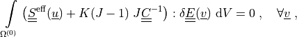
Find $\ul{u}$ such that:

$\intl{\Omega\suz}{} \left( \ull{S}\eff(\ul{u}) + K(J-1)\; J \ull{C}^{-1} \right) : \delta \ull{E}(\ul{v}) \difd{V} = 0 \;, \quad \forall \ul{v} \;,$

where

$\ull{F}$	deformation gradient $F_{ij} = \pdiff{x_i}{X_j}$
$J$	$\det(F)$
$\ull{C}$	right Cauchy-Green deformation tensor $C = F^T F$
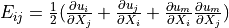
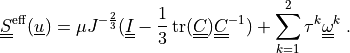
$\ull{E}(\ul{u})$	Green strain tensor $E_{ij} = \frac{1}{2}(\pdiff{u_i}{X_j} + \pdiff{u_j}{X_i} + \pdiff{u_m}{X_i}\pdiff{u_m}{X_j})$
$\ull{S}\eff(\ul{u})$	effective second Piola-Kirchhoff stress tensor

The effective stress $\ull{S}\eff(\ul{u})$ incorporates also the effects of the active fibres in two preferential directions:

$\ull{S}\eff(\ul{u}) = \mu J^{-\frac{2}{3}}(\ull{I} - \frac{1}{3}\tr(\ull{C}) \ull{C}^{-1}) + \sum_{k=1}^2 \tau^k \ull{\omega}^k \;.$

The first term is the neo-Hookean term and the sum add contributions of the two fibre systems. The tensors $\ull{\omega}^k = \ul{d}^k\ul{d}^k$ are defined by the fibre system direction vectors $\ul{d}^k$ (unit).

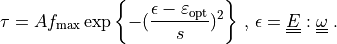
For the one-dimensional tensions $\tau^k$ holds simply ( $^k$ omitted):

$\tau = A f_{\rm max} \exp{\left\{-(\frac{\epsilon - \varepsilon_{\rm opt}}{s})^2\right\}} \mbox{ , } \epsilon = \ull{E} : \ull{\omega} \;.$

Usage Examples¶

Run with the Newton solver:

sfepy-run sfepy/examples/large_deformation/active_fibres.py

Run with the matrix-free Newton-Krylov solver from SciPy:

sfepy-run sfepy/examples/large_deformation/active_fibres.py -d solver=root

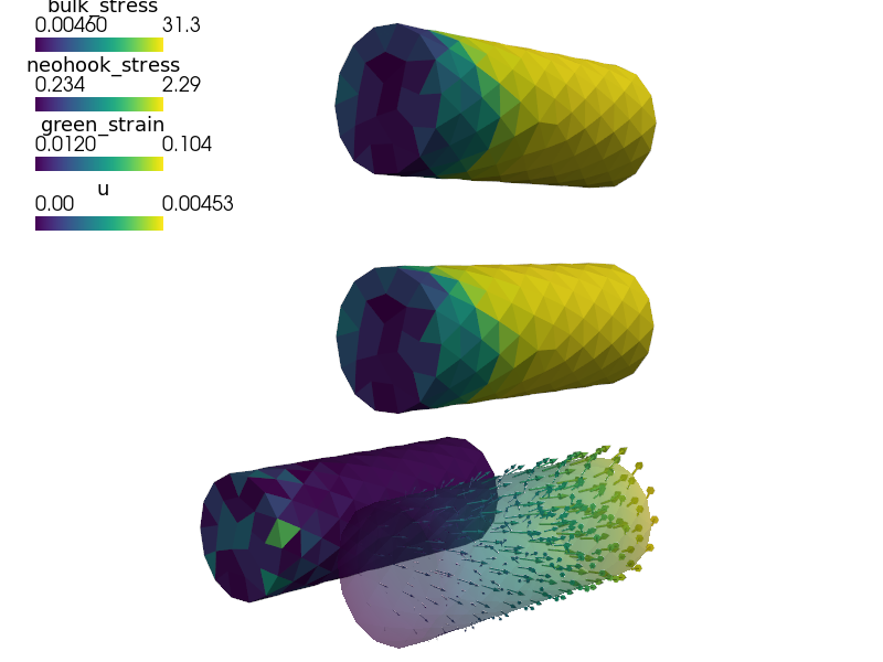
Visualize the Green strain tensor magnitude on the deforming mesh:

sfepy-view output/hsphere8.h5 -f green_strain:wu:f1:p0 1:vw:o0.3:p0 --color-limits=0.0,1.3

Visualize the stresses in active fibres on the deforming mesh:

sfepy-view output/hsphere8.h5 -f f1_stress:wu:f1:p0 1:vw:o0.3:p0 --color-limits=0,20
sfepy-view output/hsphere8.h5 -f f2_stress:wu:f1:p0 1:vw:o0.3:p0 --color-limits=0,30

sfepy-view output/hsphere8.h5 -f f1_stress:wu:f1:p0 1:vw:o0.3:p0 f2_stress:wu:f1:p1 1:vw:o0.3:p1 --grid-vector1="1.2,-1.2,0" --color-limits=0,30

../_images/large_deformation-active_fibres1.png

../_images/large_deformation-active_fibres-hsphere8-fdir0.png

../_images/large_deformation-active_fibres-hsphere8-fdir1.png

source code

# -*- coding: utf-8 -*-
r"""
Nearly incompressible hyperelastic material model with active fibres.

Large deformation is described using the total Lagrangian formulation.
Models of this kind can be used in biomechanics to model biological
tissues, e.g. muscles.

Find :math:`\ul{u}` such that:

.. math::
    \intl{\Omega\suz}{} \left( \ull{S}\eff(\ul{u})
    + K(J-1)\; J \ull{C}^{-1} \right) : \delta \ull{E}(\ul{v}) \difd{V}
    = 0
    \;, \quad \forall \ul{v} \;,

where

.. list-table::
   :widths: 20 80

   * - :math:`\ull{F}`
     - deformation gradient :math:`F_{ij} = \pdiff{x_i}{X_j}`
   * - :math:`J`
     - :math:`\det(F)`
   * - :math:`\ull{C}`
     -  right Cauchy-Green deformation tensor :math:`C = F^T F`
   * - :math:`\ull{E}(\ul{u})`
     - Green strain tensor :math:`E_{ij} = \frac{1}{2}(\pdiff{u_i}{X_j} +
       \pdiff{u_j}{X_i} + \pdiff{u_m}{X_i}\pdiff{u_m}{X_j})`
   * - :math:`\ull{S}\eff(\ul{u})`
     - effective second Piola-Kirchhoff stress tensor

The effective stress :math:`\ull{S}\eff(\ul{u})` incorporates also the
effects of the active fibres in two preferential directions:

.. math::
    \ull{S}\eff(\ul{u}) = \mu J^{-\frac{2}{3}}(\ull{I}
    - \frac{1}{3}\tr(\ull{C}) \ull{C}^{-1})
    + \sum_{k=1}^2 \tau^k \ull{\omega}^k
    \;.

The first term is the neo-Hookean term and the sum add contributions of
the two fibre systems. The tensors :math:`\ull{\omega}^k =
\ul{d}^k\ul{d}^k` are defined by the fibre system direction vectors
:math:`\ul{d}^k` (unit).

For the one-dimensional tensions :math:`\tau^k` holds simply (:math:`^k`
omitted):

.. math::
    \tau = A f_{\rm max} \exp{\left\{-(\frac{\epsilon - \varepsilon_{\rm
    opt}}{s})^2\right\}} \mbox{ , } \epsilon = \ull{E} : \ull{\omega}
    \;.

Usage Examples
--------------

- Run with the Newton solver::

    sfepy-run sfepy/examples/large_deformation/active_fibres.py

- Run with the matrix-free Newton-Krylov solver from SciPy::

    sfepy-run sfepy/examples/large_deformation/active_fibres.py -d solver=root

- Visualize the Green strain tensor magnitude on the deforming mesh::

    sfepy-view output/hsphere8.h5 -f green_strain:wu:f1:p0 1:vw:o0.3:p0 --color-limits=0.0,1.3

- Visualize the stresses in active fibres on the deforming mesh::

    sfepy-view output/hsphere8.h5 -f f1_stress:wu:f1:p0 1:vw:o0.3:p0 --color-limits=0,20
    sfepy-view output/hsphere8.h5 -f f2_stress:wu:f1:p0 1:vw:o0.3:p0 --color-limits=0,30

    sfepy-view output/hsphere8.h5 -f f1_stress:wu:f1:p0 1:vw:o0.3:p0 f2_stress:wu:f1:p1 1:vw:o0.3:p1 --grid-vector1="1.2,-1.2,0" --color-limits=0,30
"""
from functools import partial

import numpy as nm

from sfepy import data_dir
from sfepy.base.base import Struct
from sfepy.base.ioutils import edit_filename
from sfepy.homogenization.utils import define_box_regions

def get_pars_fibres(ts, coors, mode=None, which=0, vf=1.0, **kwargs):
    """
    Parameters
    ----------
    ts : TimeStepper
        Time stepping info.
    coors : array_like
        The physical domain coordinates where the parameters shound be defined.
    mode : 'qp' or 'special'
        Call mode.
    which : int
        Fibre system id.
    vf : float
        Fibre system volume fraction.
    """
    if mode != 'qp': return

    fmax = 100.0
    eps_opt = 0.01
    s = 1.0

    tt = ts.time * 2.0 * nm.pi

    x, y, z = coors[:,0], coors[:,1], coors[:,2]
    # Spherical coordinates.
    r = nm.sqrt(x**2 + y**2 + z**2)
    theta = nm.arccos(z / r)[:,None]
    phi = nm.arctan2(y, x)[:,None]
    act = 0.5 * (1.0 + nm.sin(tt - (0.5 * nm.pi)))

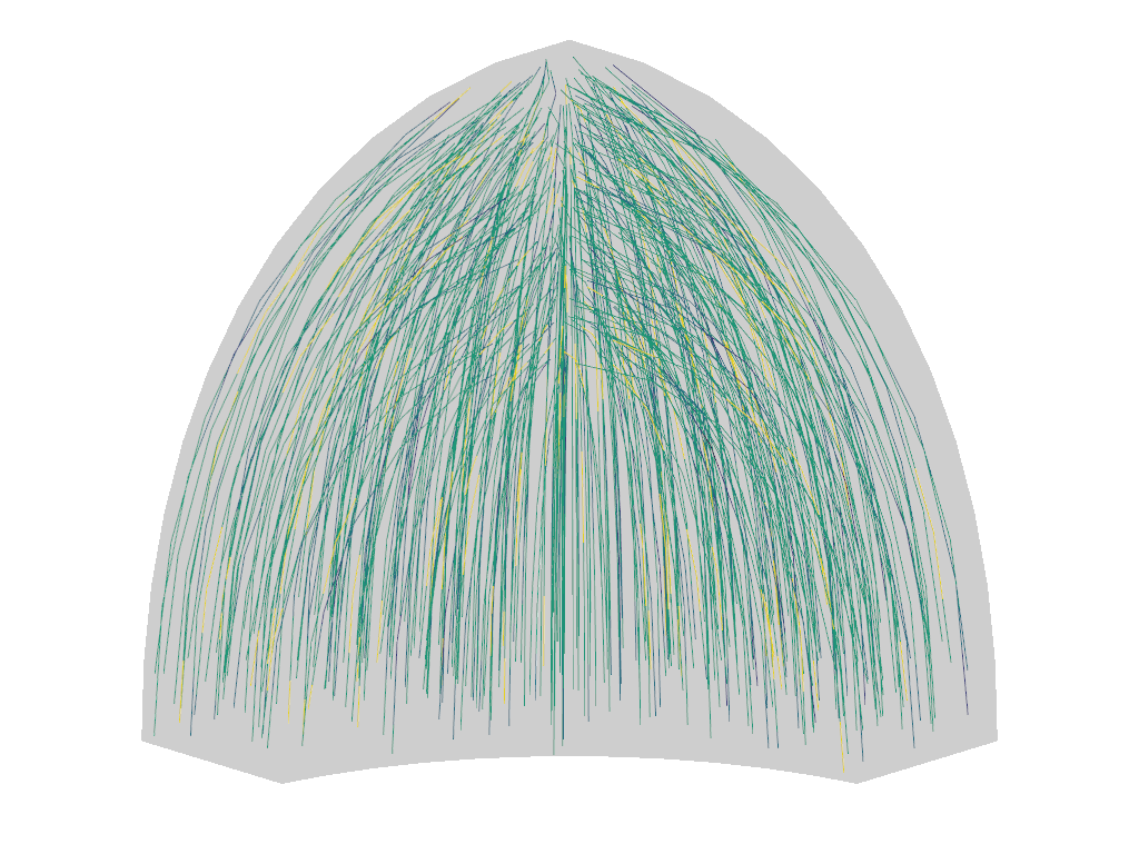
    if which == 0: # system 1 - meridians
        fdir = nm.c_[nm.cos(theta) * nm.cos(phi),
                     nm.cos(theta) * nm.sin(phi),
                     - nm.sin(theta)]

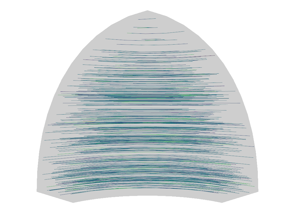
    elif which == 1: # system 2 - parallels
        fdir = nm.c_[-nm.sin(phi), nm.cos(phi), nm.zeros_like(phi)]

    else:
        raise ValueError(f'unknown fibre system {which}!')

    nfdir = nm.linalg.norm(fdir, axis=1, keepdims=True)
    fdir /= nm.where(nfdir > 0.0, nfdir, 1.0)

    shape = (coors.shape[0], 1, 1)
    out = {
        'fmax' : vf * nm.tile(fmax, shape),
        'eps_opt' : nm.tile(eps_opt, shape),
        's' : nm.tile(s, shape),
        'fdir' : fdir.reshape((coors.shape[0], 3, 1)),
        'act' : nm.tile(act, shape),
    }

    return out

def stress_strain(out, pb, state, extend=False):
    ev = partial(pb.evaluate, mode='el_avg', verbose=False)

    strain = ev('dw_tl_he_neohook.i.Omega(solid.mu, v, u)', term_mode='strain')
    out['green_strain'] = Struct(name='result', mode='cell', data=strain)

    stress = ev('dw_tl_he_neohook.i.Omega(solid.mu, v, u)', term_mode='stress')
    out['neohook_stress'] = Struct(name='result', mode='cell', data=stress)

    stress = ev('dw_tl_bulk_penalty.i.Omega(solid.K, v, u)', term_mode= 'stress')
    out['bulk_stress'] = Struct(name='output_data', mode='cell', data=stress)

    stress = ev(
        'dw_tl_fib_a.i.Omega(f1.fmax, f1.eps_opt, f1.s, f1.fdir, f1.act, v, u)',
        term_mode= 'stress',
    )
    out['f1_stress'] = Struct(name='result', mode='cell', data=stress)

    stress = ev(
        'dw_tl_fib_a.i.Omega(f2.fmax, f2.eps_opt, f2.s, f2.fdir, f2.act, v, u)',
        term_mode= 'stress',
    )
    out['f2_stress'] = Struct(name='result', mode='cell', data=stress)

    ts = pb.get_timestepper()
    if ts.step == 0:
        coors = pb.domain.get_mesh_coors()
        fout = {}
        for ii in range(2):
            aux = get_pars_fibres(ts, coors, mode='qp', which=ii, vf=1.0)
            fout[f'fdir{ii}'] = Struct(name='result', mode='vertex',
                                       data=aux['fdir'])

        filename = edit_filename(pb.get_output_name(),
                                 suffix='_fibres', new_ext='.vtk')
        pb.save_state(filename, out=fout)

    return out

def define(solver='newton', refine=0, n_step=21, output_dir='output'):
    filename_mesh = data_dir + '/meshes/3d/hsphere8.vtk'

    vf_matrix = 0.5
    vf_fibres1 = 0.2
    vf_fibres2 = 0.3

    options = {
        'nls' : solver,
        'ls' : 'ls',
        'ts' : 'ts',
        'refinement_level' : refine,
        'save_times' : 'all',
        'post_process_hook' : 'stress_strain',
        'output_format' : 'h5',
        'output_dir' : output_dir,
    }

    fields = {
        'displacement': (nm.float64, 3, 'Omega', 1),
    }

    materials = {
        'solid' : ({
            'K'  : vf_matrix * 1e3, # bulk modulus
            'mu' : vf_matrix * 20e0, # shear modulus of neoHookean term
        },),
        'f1' : 'get_pars_fibres1',
        'f2' : 'get_pars_fibres2',
    }

    functions = {
        'get_pars_fibres1' : (lambda ts, coors, mode=None, **kwargs:
                              get_pars_fibres(ts, coors, mode=mode, which=0,
                                              vf=vf_fibres1, **kwargs),),
        'get_pars_fibres2' : (lambda ts, coors, mode=None, **kwargs:
                              get_pars_fibres(ts, coors, mode=mode, which=1,
                                              vf=vf_fibres2, **kwargs),),
    }

    variables = {
        'u' : ('unknown field', 'displacement', 0),
        'v' : ('test field', 'displacement', 'u'),
    }

    dim = 3
    bbox = [[0] * dim, [25e-6] * dim]
    bregions = define_box_regions(dim, bbox[0], bbox[1])
    regions = {
        'Omega' : 'all',
        'Left' : bregions['Left'],
        'Near' : bregions['Near'],
        'Bottom' : bregions['Bottom'],
    }

    ebcs = {
        'e0' : ('Left', {'u.0' : 0.0}),
        'e1' : ('Near', {'u.1' : 0.0}),
        'e2' : ('Bottom', {'u.2' : 0.0}),
    }

    integrals = {
        'i' : 2,
    }
    equations = {
        'balance' : """
            dw_tl_he_neohook.i.Omega(solid.mu, v, u)
          + dw_tl_bulk_penalty.i.Omega(solid.K, v, u)
          + dw_tl_fib_a.i.Omega(f1.fmax, f1.eps_opt, f1.s, f1.fdir, f1.act, v, u)
          + dw_tl_fib_a.i.Omega(f2.fmax, f2.eps_opt, f2.s, f2.fdir, f2.act, v, u)
          = 0
        """,
    }

    solvers = {
        'ls' : ('ls.auto_direct', {}),
        'newton' : ('nls.newton', {
            'i_max'      : 10,
            'eps_a'      : 0.0,
            'eps_r'      : 1e-5,
            'eps_mode'   : 'or',
            'macheps'    : 1e-16,
            'lin_red'    : None, # Linear system error < (eps_a * lin_red).
            'ls_red'     : 0.1,
            'ls_red_warp': 0.001,
            'ls_on'      : 10.0,
            'ls_min'     : 1e-5,
            'check'      : 0,
            'delta'      : 1e-6,
            'report_status' : True,
        }),
        'root' : ('nls.scipy_root', {
            'method' : 'krylov',
            'use_jacobian' : False,
            'report_status' : True,
            'options' : {
                'ftol' : 1e-3,
            },
        }),
        'ts' : ('ts.simple', {
            't0' : 0.0,
            't1' : 1.0 * n_step / 21.0,
            'dt' : None,
            'quasistatic' : True,
            'n_step' : n_step, # has precedence over dt.
            'verbose' : 1,
        }),
    }

    return locals()