diffusion/time_heat_equation_multi_material.py¶

Description

Transient heat equation with time-dependent source term, three different material domains and Newton type boundary condition loss term.

Description¶

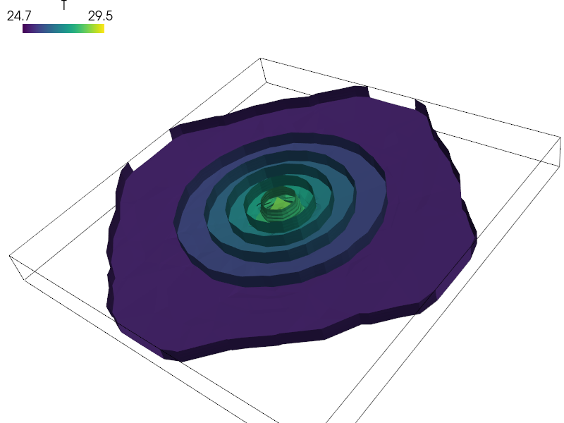
This example is inspired by the Laser Powder Bed Fusion additive manufacturing process. A laser source deposits a flux on a circular surface (a full layer of the cylinder being built) at regular time intervals. The heat propagates into the build plate and to the sides of the cylinder into powder which is relatively bad at conductiong heat. Heat losses through Newton type heat exchange occur both at the surface where the heat is being deposited and at the bottom plate.

The PDE for this physical process implies to find $T(x, t)$ for $x \in \Omega, t \in [0, t_{\rm final}]$ such that:

$\left\lbrace \begin{aligned} \rho(x)c_p(x)\frac{\partial T}{\partial t}(x, t) = -\nabla \cdot \left( -k(x) \underline{\nabla} T(x, t) \right) && \forall x \in \Omega, \forall t \in [0, T_{max}] \\ -k \underline{\nabla} T(x, t)\cdot \underline{n} = q(t)+h(T-T_\infty) && \forall x \in \Gamma_{source} \\ -k \underline{\nabla} T(x, t)\cdot \underline{n} = q(t)+h(T-T_\infty) && \forall x \in \Gamma_{plate} \\ \underline{\nabla} T(x, t)\cdot \underline{n} = 0 && \forall x \in \Gamma \setminus(\Gamma_{source} \cap\Gamma_{plate}) \end{aligned} \right.$

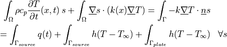
The weak formulation solved using sfepy is to find a discretized field $T$ that satisfies:

$\begin{aligned} \int_\Omega\rho c_p \frac{\partial T}{\partial t}(x, t) \, s + \int_\Omega \underline{\nabla} s \cdot (k(x) \underline{\nabla} T) = \int_\Gamma -k \underline{\nabla} T \cdot \underline{n} s \\ = \int_{\Gamma_{source}} q(t) + \int_{\Gamma_{source}} h(T-T_\infty) + \int_{\Gamma_{plate}} h(T-T_\infty) && \forall s \end{aligned}$

Uniform initial conditions are used as a starting point of the simulation.

Usage examples¶

The script can be run with:

sfepy-run sfepy/examples/diffusion/time_heat_equation_multi_material.py

The last time-step result field can then be visualized as isosurfaces with:

sfepy-view multi_material_cylinder_plate.119.vtk -i 10 -l

The resulting time evolution of temperatures is saved as an image file in the output directory (heat_probe_time_evolution.png).

This script uses SI units (meters, kilograms, Joules…) except for temperature, which is expressed in degrees Celsius.

../_images/diffusion-time_heat_equation_multi_material.png

source code

r"""
Transient heat equation with time-dependent source term, three different
material domains and Newton type boundary condition loss term.

Description
-----------

This example is inspired by the Laser Powder Bed Fusion additive manufacturing
process. A laser source deposits a flux on a circular surface (a full layer of
the cylinder being built) at regular time intervals. The heat propagates into
the build plate and to the sides of the cylinder into powder which is
relatively bad at conductiong heat. Heat losses through Newton type heat
exchange occur both at the surface where the heat is being deposited and at the
bottom plate.

The PDE for this physical process implies to find :math:`T(x, t)` for :math:`x
\in \Omega, t \in [0, t_{\rm final}]` such that:

.. math::
    \left\lbrace
    \begin{aligned}
    \rho(x)c_p(x)\frac{\partial T}{\partial t}(x, t)
    = -\nabla \cdot \left( -k(x) \underline{\nabla} T(x, t) \right) &&
    \forall x \in \Omega, \forall t \in [0, T_{max}] \\
    -k \underline{\nabla} T(x, t)\cdot \underline{n}
    = q(t)+h(T-T_\infty) && \forall x \in \Gamma_{source} \\
    -k \underline{\nabla} T(x, t)\cdot \underline{n}
    = q(t)+h(T-T_\infty) && \forall x \in \Gamma_{plate} \\
    \underline{\nabla} T(x, t)\cdot \underline{n}
    = 0 && \forall x \in \Gamma \setminus(\Gamma_{source}
    \cap\Gamma_{plate})
    \end{aligned}
    \right.

The weak formulation solved using `sfepy` is to find a discretized field
:math:`T` that satisfies:

.. math::
    \begin{aligned}
    \int_\Omega\rho c_p \frac{\partial T}{\partial t}(x, t) \, s
    + \int_\Omega \underline{\nabla} s \cdot (k(x)
    \underline{\nabla}
    T) =  \int_\Gamma -k \underline{\nabla} T \cdot \underline{n} s \\
    = \int_{\Gamma_{source}} q(t)   +
    \int_{\Gamma_{source}} h(T-T_\infty)
    + \int_{\Gamma_{plate}} h(T-T_\infty)  && \forall s
    \end{aligned}

Uniform initial conditions are used as a starting point of the simulation.

Usage examples
--------------
The script can be run with::

    sfepy-run sfepy/examples/diffusion/time_heat_equation_multi_material.py

The last time-step result field can then be visualized as isosurfaces with::

    sfepy-view multi_material_cylinder_plate.119.vtk -i 10 -l

The resulting time evolution of temperatures is saved as an image file in the
output directory (heat_probe_time_evolution.png).

This script uses SI units (meters, kilograms, Joules...) except for
temperature, which is expressed in degrees Celsius.
"""
import numpy as nm
from sfepy import data_dir
from sfepy.discrete.probes import LineProbe
import matplotlib.pyplot as plt
import os

nominal_heat_flux = 6.36e5
alpha = 0.25
t_start = nm.array([0., 20., 40.])  # times when heating starts (seconds)
t_stop = nm.array([10., 30., 50.])  # times when heating stops (seconds)

T0 = 25.  # °C
h = 50.  # W/m2/K
mm = 1e-3

filename_mesh = data_dir + '/meshes/3d/multi_material_cylinder_plate.vtk'

materials = {
    'powder': ({'lam': 0.16,
                'rho_cp': 1330. * 650.},),
    'cylinder': ({'lam': 153.,
                  'rho_cp': 2760. * 935.,
                  'lam_vec': 173. * nm.eye(3)},),
    'plate': ({'lam': 153.,
               'rho_cp': 2660. * 927.,
               'lam_vec': 153. * nm.eye(3)},),

    'heat_flux_defined_by_func': 'get_flux_value',
    'heat_loss': ({'h_bot': -h, 'T_bot_inf': T0,
                   'h_top': -h, 'T_top_inf': T0},)
}

regions = {
    'Omega': 'all',
    'Omega_Cylinder': 'cells of group 4',
    'Omega_Powder': 'cells of group 3',
    'Omega_Plate': 'cells of group 1 +v cells of group 2',
    'Gamma_Plate': ('vertices in (z < -9.95e-3)', 'facet'),
    'Gamma_Source': ('vertices of surface *v r.Omega_Cylinder', 'face'),
}


def get_flux_value(ts, coors, mode=None, **kwargs):
    """Defines heat flux as a function of time."""
    if mode == 'qp':
        shape = (coors.shape[0], 1, 1)
        if nm.any((ts.time >= t_start) & (ts.time <= t_stop)):
            flux = alpha * nominal_heat_flux
        else:
            flux = 0.
        val = flux * nm.ones(shape, dtype=nm.float64)
        return {'val': val}


functions = {
    'get_flux_value': (get_flux_value,),
}

fields = {
    'temperature': ('real', 1, 'Omega', 1),
}

variables = {
    'T': ('unknown field', 'temperature', 1, 1),  # 1 means history=1
    's': ('test field', 'temperature', 'T'),
}

ebcs = {
}

integrals = {
    'i': 2
}

equations = {
    'Temperature': """
      dw_dot.i.Omega_Cylinder(cylinder.rho_cp, s, dT/dt )
    + dw_dot.i.Omega_Plate(plate.rho_cp, s, dT/dt )
    + dw_dot.i.Omega_Powder(powder.rho_cp, s, dT/dt )
    + dw_laplace.i.Omega_Cylinder(cylinder.lam, s, T)
    + dw_laplace.i.Omega_Plate(plate.lam, s, T)
    + dw_laplace.i.Omega_Powder(powder.lam, s, T)
    = dw_integrate.i.Gamma_Source(heat_flux_defined_by_func.val, s)
    + dw_bc_newton.i.Gamma_Source(heat_loss.h_top, heat_loss.T_top_inf, s, T)
    + dw_bc_newton.i.Gamma_Plate(heat_loss.h_bot, heat_loss.T_bot_inf, s, T)
    """
}

ics = {
    'ic1': ('Omega_Powder', {'T.0': T0}),
    'ic2': ('Omega_Plate', {'T.0': T0}),
    'ic3': ('Omega_Cylinder', {'T.0': T0}),
}


def gen_probe():
    """Instantiates a line probe used later by the `step_hook` function."""
    p0, p1 = nm.array([0., 0., -10. * mm]), nm.array([0.0, 0.0, 15. * mm])
    line_probe = LineProbe(p0, p1, n_point=100, share_geometry=True)
    return line_probe


line_probe = gen_probe()
# inits an empty list that will hold the probe results
probe_results = []


def step_hook(pb, ts, variables):
    """
    This implements a function that gets called at every step from the
    time-solver.
    """
    T_field = pb.get_variables()['T']
    pars, vals = line_probe(T_field)
    probe_results.append(vals)


def post_process_hook(out, pb, state, extend=False):
    ts = pb.ts
    if ts.step == ts.n_step - 1:
        fig, (ax1, ax2) = plt.subplots(nrows=2)
        temperature_image = nm.array(probe_results).squeeze()
        m = ax1.imshow(temperature_image.T, origin='lower', aspect='auto')
        ax1.set_xlabel("time step")
        ax1.set_ylabel("distance across build\nplate and cylinder")
        fig.colorbar(m, ax=ax1, label="temperature")
        ax2.plot(temperature_image.T[0], label="bottom")
        ax2.plot(temperature_image.T[-1], label="top")
        ax2.set_xlabel("time step")
        ax2.set_ylabel("temperature (°C)")
        ax2.legend()
        fig.tight_layout()
        fig.savefig(os.path.join(pb.output_dir, 'heat_probe_time_evolution.png'),
                    bbox_inches='tight')
    return out


solvers = {
    'ls': ('ls.auto_direct', {
        # Reuse the factorized linear system from the first time step.
        'use_presolve': True,
        # Speed up the above by omitting the matrix digest check used normally
        # for verification that the current matrix corresponds to the
        # factorized matrix stored in the solver instance. Use with care!
        'use_mtx_digest': False,
    }),
    'newton': ('nls.newton', {
        'i_max': 1,
        'eps_a': 1e-5,
        'is_linear': True,
    }),
    'ts': ('ts.simple', {
        't0': 0.0,
        't1': 60.,
        'dt': None,
        'n_step': 120,
        'verbose': True,
        'is_linear': True,
    }),
}

options = {
    'step_hook': 'step_hook',
    'post_process_hook': 'post_process_hook',
}