diffusion/poisson_nonlinear_parametric.py¶

Description

Nonlinear diffusion with a field-dependent coefficient and parametric sweep.

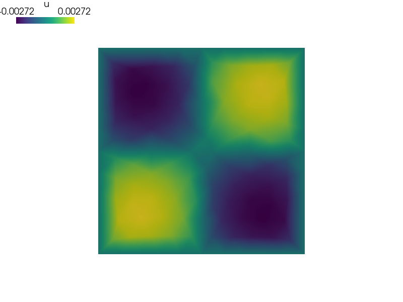
Solve the problem:

$-\nabla \cdot \left( (1 + \alpha u^2)\nabla u \right) = \sin(\pi x)\sin(\pi y) \quad \text{in } \Omega,$

with homogeneous Dirichlet boundary conditions:

$u = 0 \quad \text{on } \partial \Omega.$

The diffusion coefficient depends on the solution:

$c(u) = 1 + \alpha u^2.$

The problem is solved for several values of $\alpha$ , and the solutions are compared to the linear case $\alpha = 0$ .

Usage Examples¶

Run with the default parameters:

sfepy-run sfepy/examples/diffusion/poisson_nonlinear_parametric.py
sfepy-view output/poisson_nonlinear_parametric/square_unit_tri_alpha_*.vtk -2

Use custom values of $\alpha$ , show $\nabla u$ :

sfepy-run sfepy/examples/diffusion/poisson_nonlinear_parametric.py -d "alphas=[1e5,5e5,1e6]"
sfepy-view output/poisson_nonlinear_parametric/square_unit_tri_alpha_*.vtk -2 -f u:gu:p0 u:p0 --no-scalar-bars

../_images/diffusion-poisson_nonlinear_parametric.png

source code

r"""
Nonlinear diffusion with a field-dependent coefficient and parametric sweep.

Solve the problem:

.. math::

   -\nabla \cdot \left( (1 + \alpha u^2)\nabla u \right)
   = \sin(\pi x)\sin(\pi y)
   \quad \text{in } \Omega,

with homogeneous Dirichlet boundary conditions:

.. math::

   u = 0 \quad \text{on } \partial \Omega.

The diffusion coefficient depends on the solution:

.. math::

   c(u) = 1 + \alpha u^2.

The problem is solved for several values of :math:`\alpha`, and the
solutions are compared to the linear case :math:`\alpha = 0`.

Usage Examples
--------------

- Run with the default parameters::

    sfepy-run sfepy/examples/diffusion/poisson_nonlinear_parametric.py
    sfepy-view output/poisson_nonlinear_parametric/square_unit_tri_alpha_*.vtk -2

- Use custom values of :math:`\alpha`, show :math:`\nabla u`::

    sfepy-run sfepy/examples/diffusion/poisson_nonlinear_parametric.py -d "alphas=[1e5,5e5,1e6]"
    sfepy-view output/poisson_nonlinear_parametric/square_unit_tri_alpha_*.vtk -2 -f u:gu:p0 u:p0 --no-scalar-bars
"""
from sfepy import data_dir
from sfepy.base.base import output
import numpy as nm

def define(alphas=None, order=1, qp_order=4, i_max=20,
           output_dir='output/poisson_nonlinear_parametric'):
    filename_mesh = data_dir + '/meshes/2d/square_unit_tri.mesh'
    if alphas is None:
        alphas = [0, 1000, 10000, 100000, 1000000]
    _state = {'alpha': 0.0}
    def conductivity(u):
        val = 1.0 + _state['alpha'] * u**2
        return val

    def d_conductivity(u):
        # derivative of (1 + alpha * u^2) w.r.t. u
        return 2.0 * _state['alpha'] * u

    def get_rhs(ts, coors, mode=None, **kwargs):
        if mode == 'qp':
            x = coors[:, 0]
            y = coors[:, 1]
            val = nm.sin(nm.pi * x) * nm.sin(nm.pi * y)
            val = val.reshape((-1, 1, 1))
            return {'val': val}

    def vary_alpha(problem):
        baseline = None

        ofn_trunk = problem.ofn_trunk
        output_format = problem.output_format
        output_dir = problem.output_dir

        # Newton handles the nonlinearity; we just sweep alpha values
        for alpha in alphas:
            _state['alpha'] = alpha

            alpha_tag = f'{alpha:010.2f}'.replace('.', '_')
            problem.setup_output(
                output_filename_trunk=ofn_trunk + '_alpha_' + alpha_tag,
                output_dir=output_dir,
                output_format=output_format,
            )
            yield problem, []
            vec = problem.get_variables()['u']().copy()
            if baseline is None:
                baseline = vec.copy()
            diff_norm = nm.linalg.norm(vec - baseline)
            sol_norm = nm.linalg.norm(vec)
            output('---')
            output('alpha:', alpha, '||u||:', sol_norm, '||u - u0||:', diff_norm)
            yield

    materials = {
        'rhs': 'get_rhs',
    }

    fields = {
        'fu': ('real', 1, 'Omega', order),
    }

    variables = {
        'u': ('unknown field', 'fu', 0),
        'v': ('test field', 'fu', 'u'),
    }

    regions = {
        'Omega': 'all',
        'Gamma': ('vertices of surface', 'facet'),
    }

    ebcs = {
        'u0': ('Gamma', {'u.0': 0.0}),
    }

    functions = {
        'get_rhs': (get_rhs,),
        'conductivity': (conductivity,),
        'd_conductivity': (d_conductivity,),
    }

    integrals = {
        'i': qp_order,
    }

    equations = {
        'Balance': """
            dw_nl_diffusion.i.Omega( conductivity, d_conductivity, v, u )
            = dw_volume_lvf.i.Omega( rhs.val, v )
        """
    }

    solvers = {
        'ls': ('ls.scipy_direct', {}),
        'newton': ('nls.newton', {
            'i_max': i_max,
            'eps_a': 1e-10,
            'eps_r': 1.0,
        }),
    }

    options = {
        'nls': 'newton',
        'ls': 'ls',
        'parametric_hook': 'vary_alpha',
        'output_dir': output_dir,
    }

    return locals()