diffusion/laplace_fluid_2d.py¶

Description

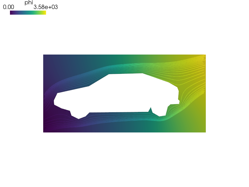
A Laplace equation that models the flow of “dry water” around an obstacle shaped like a Citroen CX.

Description¶

As discussed e.g. in the Feynman lectures Section 12-5 of Volume 2 (https://www.feynmanlectures.caltech.edu/II_12.html#Ch12-S5), the flow of an irrotational and incompressible fluid can be modelled with a potential $\ul{v} = \ul{grad}(\phi)$ that obeys

$\nabla \cdot \ul{\nabla}\,\phi = \Delta\,\phi = 0$

The weak formulation for this problem is to find $\phi$ such that:

$\int_{\Omega} \nabla \psi \cdot \nabla \phi = \int_{\Gamma_{left}} \ul{v}_0 \cdot n \, \psi + \int_{\Gamma_{right}} \ul{v}_0 \cdot n \, \psi + \int_{\Gamma_{top}} \ul{v}_0 \cdot n \,\psi + \int_{\Gamma_{bottom}} \ul{v}_0 \cdot n \, \psi \;, \quad \forall \psi \;,$

where $\ul{v}_0$ is the 2D vector defining the far field velocity that generates the incompressible flow.

Since the value of the potential is defined up to a constant value, a Dirichlet boundary condition is set at a single vertex to avoid having a singular matrix.

Usage examples¶

This example can be run with the following:

sfepy-run sfepy/examples/diffusion/laplace_fluid_2d.py
sfepy-view citroen.vtk -f phi:p0 phi:t50:p0 --2d-view

Generating the mesh¶

The mesh can be generated with:

gmsh -2 -f msh22 meshes/2d/citroen.geo -o meshes/2d/citroen.msh
sfepy-convert --2d meshes/2d/citroen.msh meshes/2d/citroen.h5

../_images/diffusion-laplace_fluid_2d.png

source code

r"""
A Laplace equation that models the flow of "dry water" around an obstacle
shaped like a Citroen CX.


Description
-----------

As discussed e.g. in the Feynman lectures Section 12-5 of Volume 2
(https://www.feynmanlectures.caltech.edu/II_12.html#Ch12-S5),
the flow of an irrotational and incompressible fluid can be modelled with a
potential :math:`\ul{v} = \ul{grad}(\phi)` that obeys

.. math::
    \nabla \cdot \ul{\nabla}\,\phi = \Delta\,\phi = 0

The weak formulation for this problem is to find :math:`\phi` such that:

.. math::
    \int_{\Omega} \nabla \psi \cdot \nabla \phi
    = \int_{\Gamma_{left}} \ul{v}_0 \cdot n  \, \psi
    + \int_{\Gamma_{right}} \ul{v}_0 \cdot n  \, \psi
    + \int_{\Gamma_{top}} \ul{v}_0 \cdot n \,\psi
    + \int_{\Gamma_{bottom}} \ul{v}_0 \cdot n \, \psi
    \;, \quad \forall \psi \;,

where :math:`\ul{v}_0` is the 2D vector defining the far field velocity that
generates the incompressible flow.

Since the value of the potential is defined up to a constant value, a Dirichlet
boundary condition is set at a single vertex to avoid having a singular matrix.

Usage examples
--------------

This example can be run with the following::

  sfepy-run sfepy/examples/diffusion/laplace_fluid_2d.py
  sfepy-view citroen.vtk -f phi:p0 phi:t50:p0 --2d-view

Generating the mesh
-------------------

The mesh can be generated with::

  gmsh -2 -f msh22 meshes/2d/citroen.geo -o meshes/2d/citroen.msh
  sfepy-convert --2d meshes/2d/citroen.msh meshes/2d/citroen.h5
"""
import numpy as nm
from sfepy import data_dir

filename_mesh = data_dir + '/meshes/2d/citroen.h5'

v0 = nm.array([1, 0.25])

materials = {
    'm': ({'v0': v0.reshape(-1, 1)},),
}

regions = {
    'Omega': 'all',
    'Gamma_Left': ('vertices in (x < 0.1)', 'facet'),
    'Gamma_Right': ('vertices in (x > 1919.9)', 'facet'),
    'Gamma_Top': ('vertices in (y > 917.9)', 'facet'),
    'Gamma_Bottom': ('vertices in (y < 0.1)', 'facet'),
    'Vertex': ('vertex in r.Gamma_Left', 'vertex'),
}

fields = {
    'u': ('real', 1, 'Omega', 1),
}

variables = {
    'phi': ('unknown field', 'u', 0),
    'psi': ('test field', 'u', 'phi'),
}

# these EBCS prevent the matrix from being singular, see description
ebcs = {
    'fix': ('Vertex', {'phi.0': 0.0}),
}

integrals = {
    'i': 2,
}

equations = {
    'Laplace equation':
        """dw_laplace.i.Omega( psi, phi )
         = dw_surface_ndot.i.Gamma_Left( m.v0, psi )
         + dw_surface_ndot.i.Gamma_Right( m.v0, psi )
         + dw_surface_ndot.i.Gamma_Top( m.v0, psi )
         + dw_surface_ndot.i.Gamma_Bottom( m.v0, psi )"""
}

solvers = {
    'ls': ('ls.scipy_direct', {}),
    'newton': ('nls.newton', {
        'i_max': 1,
        'eps_a': 1e-10,
    }),
}