Numerical simulation of fluid-saturated piezoelectric porous media
Mathematical model
We consider a porous piezoelectric medium which consists of a piezoelectric matrix, embedded metallic electrodes (conductors) and fluid-filled inclusions. These components are arranged in a periodic lattice so that the medium can be generated by copies of the reference unit cell, see Fig. 1. The mechanical behavior of such a structure can be described using the two-scale asymptotic homogenization method, see [RohanLukes2018].
The mechanical properties of the piezoelectric solid are given by the following constitutive equations
(1)
where  is the Cauchy stress tensor,
  is the electric displacement,
 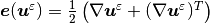 is the strain
tensor,
is the strain
tensor,  is the displacement field,
 is the electric field and
 is the electric potential. On the right hand side of
(1), we have the fourth-order elastic tensor
is the electric potential. On the right hand side of
(1), we have the fourth-order elastic tensor
 (
( ), the third-order tensor
  (
( ), which couples mechanical and electric
quantities, and the permeability tensor
), which couples mechanical and electric
quantities, and the permeability tensor  .
The superscript
.
The superscript  denotes the quantities oscillating within the heterogeneous
structure with the period equal to the size of the periodic unit.
denotes the quantities oscillating within the heterogeneous
structure with the period equal to the size of the periodic unit.
The quasi-static problem of the piezoelectric medium is given by the following equilibrium equations
(2)
end by the mass conservation equation for the k th fluid inclusion occupying
domain 
(3)
where  is the inclusion pressure and
  is the
fluid compressibility.
is the
fluid compressibility.
Two-scale homogenization
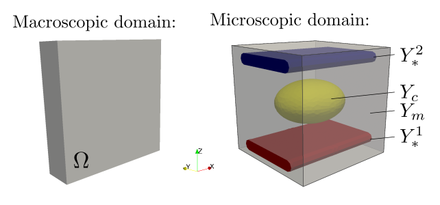
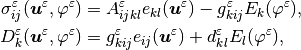
Fig. 1 Macroscopic domain  and decomposition of microscopic domain
We apply the standard homogenization techniques to the above problem. It
results in the limit model for  , where
 is the scale parameter relating the microscopic and macroscopic
length scales. The homogenization process leads to local microscopic problems,
defined within a reference periodic cell, and to the global problem describing
the behavior of the homogenized medium at the macroscopic level. The global
problem involves the homogenized material coefficients which are evaluated
using the solutions of the local problems. Due to linearity of the problem, the
microscopic and macroscopic problems are decoupled.
is the scale parameter relating the microscopic and macroscopic
length scales. The homogenization process leads to local microscopic problems,
defined within a reference periodic cell, and to the global problem describing
the behavior of the homogenized medium at the macroscopic level. The global
problem involves the homogenized material coefficients which are evaluated
using the solutions of the local problems. Due to linearity of the problem, the
microscopic and macroscopic problems are decoupled.
As we assume given potentials  in each of the electrode networks,
the dielectric properties must be appropriately rescaled in order to preserve
the finite electric field in the limit:
in each of the electrode networks,
the dielectric properties must be appropriately rescaled in order to preserve
the finite electric field in the limit:
(4)
The local microscopic responses of the piezoelectric structure are given by the
following sub-problems which are solved within the periodic reference cell ,
see Fig. 1, that is decomposed similarly to the decomposition of
domain :
Find
 ,
,  such that for all
  ,
,  and for any
(5)¶![\int_{Y_{m*}} \left[\Ab \eeb{\omegab^{ij} + \Pib^{ij}}\right]: \eeb{\vb}\,\dV - \int_{Y_m} \left[\bar\gb^T\cdot\nabla \eta^{ij}\right]: \eeb{\vb} \, \dV &= 0, \\
\int_{Y_m} \left[\bar\gb:\eeb{\omegab^{ij} + \Pib^{ij}} + \bar\db \cdot\nabla \eta^{ij}\right]\cdot\nabla\psi \, \dV &= 0,](_images/math/d9e35e1feec11a9a689df735093c18c52b973391.png)
where  .
.
Find
 ,
,  such that for all ,
satisfying
such that for all ,
satisfying
(6)¶![\int_{Y_{m*}} \left[\Ab \eeb{\omegab^P}\right]: \eeb{\vb}\,\dV - \int_{Y_m} \left[\bar\gb^T\cdot\nabla \eta^P\right]: \eeb{\vb} \,\dV &= -{1\over \vert Y\vert}\int_{\Gamma_c} \vb \cdot \nb\, \dS , \\
\int_{Y_m} \left[\bar\gb:\eeb{\omegab^P} + \bar\db \cdot\nabla \eta^P\right]\cdot\nabla\psi \,\dV &= 0.](_images/math/8299772372e45394e5ca0e77b99974cfcf520b2f.png)
Find
 ,
,  such that for all ,
satisfying
such that for all ,
satisfying
(7)¶![\int_{Y_{m*}} \left[\Ab \eeb{\omegab^\rho}\right]: \eeb{\vb}\,\dV - \int_{Y_m} \left[\bar\gb^T\cdot\nabla \eta^\rho\right]: \eeb{\vb} \,\dV &= 0 , \\
\int_{Y_m} \left[\bar\gb:\eeb{\omegab^\rho} + \bar\db \cdot\nabla \eta^\rho\right]\cdot\nabla\psi \,\dV &= -{1\over \vert Y\vert}\int_{\Gamma_{m*}} \psi\, \dS.](_images/math/c974021937c721c9564148184c758708a195ffd3.png)
Find
 ,
,  such that for all ,
and for any
such that for all ,
and for any  (
( is the number of conductors)
(8)¶![\int_{Y_{m*}} \left[\Ab \eeb{\hat\omegab^{k}}\right]: \eeb{\vb}\,\dV - \int_{Y_m} \left[\bar\gb^T\cdot\nabla \hat\eta^k\right]: \eeb{\vb} \,\dV &= 0, \\
\int_{Y_m} \left[\bar\gb:\eeb{\hat\omegab^k} + \bar\db \cdot\nabla \hat\eta^k\right]\cdot\nabla\psi \,\dV &= 0.](_images/math/793337ffbe6e338a26423c9a925379b4c0eec2b9.png)
The microscopic sub-problems are solved with the periodic boundary conditions
and  on
on  for
for 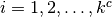 ,
,
 is the interface between
the matrix part
is the interface between
the matrix part  and
and  -th conductor
  .
Functions , and
are equal to zero on
.
Functions , and
are equal to zero on  .
.
With the characteristic responses obtained by solving local sub-problems,
the homogenized material coefficients  ,
,  ,
,  ,
,  and
and  can be evaluated
using the following expressions:
can be evaluated
using the following expressions:
(9)¶![A_{ijkl}^H & = {1\over \vert Y\vert} \left[\int_{Y_{m*}} \left[\Ab \eeb{\omegab^{ij} + \Pib^{ij}}\right]: \eeb{\omegab^{kl} + \Pib^{kl}}\,\dV
+ \int_{Y_m} \bar\db \nabla\eta^{ij} \cdot\nabla\eta^{kl}\,\dV\right],\\
B_{ijkl}^H & = {1\over \vert Y\vert} \left[\int_{Y_{m*}} \left[\Ab \eeb{\omega^{P}}\right]: \eeb{\Pib^{kl}}\,\dV
- \int_{Y_m} \bar\gb \nabla \Pib^{ij} \cdot\nabla\eta^{P}\,\dV\right] + \Phi \delta_{ij},\\
H^{H,k}_{ij} & = {1\over \vert Y\vert} \left[\int_{Y_{m*}} \left[\Ab \eeb{\hat\omegab^k}\right]: \eeb{\Pib^{ij}}\,\dV
- \int_{Y_m} \left[\bar\gb:\eeb{\Pib^{ij}}\right]\cdot\nabla\hat\eta^k\,\dV\right],\\
M^H & = {1\over \vert Y\vert} \left[\int_{Y_{m*}} \left[\Ab \eeb{\omega^{P}}\right]: \eeb{\omega^{P}}\,\dV
+ \int_{Y_m} \bar\db \nabla\eta^{P} \cdot\nabla\eta^{P}\,\dV\right] + \Phi \delta_{ij},\\
Z^{H,k} &= -{1\over \vert Y\vert}\int_{\Gamma_c} \hat\omega^k \cdot \nb\, \dS](_images/math/09fa253dfceb665614f14a68d40804d78a76678c.png)
The global macroscopic problem is defined in terms of the homogenized
coefficients as: Find the macroscopic displacements  and
and
 such that for all
  and
and 
(10)¶![\int_{\Omega} [\Ab^H \eeb{\ub^0} - p^0 \Bb^H]: \eeb{\vb}\,\dV
&= - \int_{\Omega} \eeb{\vb} : \sum\limits_k \Hb^{H,k} \bar\vphi^k \,\dV
+ \int_{\Omega} f \cdot \vb \dV,\\
\int_{\Omega} q^0(\Bb^H:\eeb{\ub^0} + p^0 M^H) \dV
&= \int_{\Omega} q^0 \sum\limits_k Z^{H,k} \bar\vphi^k \,\dV.](_images/math/c4df70360acd7b0076610930cf970afd450ddc51.png)
We assumed that the volume electric charge is equal to zero, otherwise we would need extra coefficients and right hand side terms.
Numerical simulation
To run the numerical simulation, download the archive, unpack it in the main SfePy directory and type:
./simple.py example_poropiezo-1/poropiezo_macro_dfc.py
This invoke the simply.py script which calculates the macroscopic
problem (10) and calls the homogenization engine that solves the
local subproblems (5)–(6), evaluates the homogenized
coefficients (9) and finally performs the reconstruction of the
solutions at the microscopic level. See [CimrmanLukesRohan2019] for more details related
to the SfePy homogenization engine.
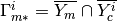
The macroscopic sample is fixed on its left side, so that no displacements are
allowed, see Fig. 2 left. The defromation is induced due to piezoelectric
effect, as the responce to the prescribed electric potentials
 ,
,  , see (10).
Fig. 2 Left - boundary conditions applied at the macroscopic level; right - revocered part of the macroscopic sample
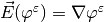
The deformed shape of the sample, pressure field  and the magnitude of
macroscopic strain
and the magnitude of
macroscopic strain  are depicted in
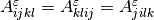
Fig. 3. The reconstructed strain and electric fields for a
given
are depicted in
Fig. 3. The reconstructed strain and electric fields for a
given  in the part of the macroscopic domain are shown in
Fig. 4.
in the part of the macroscopic domain are shown in
Fig. 4.
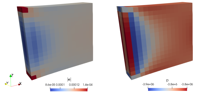
Fig. 3 Deformed macroscopic sample and the resulting fields: left - pressure
; right - magnitude of macroscopic strain  
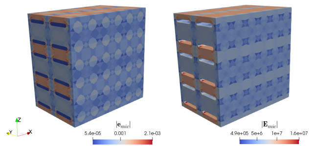
Fig. 4 Magnitudes of reconstructed fields: left - strain field  ;
right - electric field
;
right - electric field  
References
- RohanLukes2018
Rohan E., Lukeš V. Homogenization of the fluid-saturated piezoelectric porous media. International Journal of Solids and Structures, 147:110-120, 2018, DOI:10.1016/j.ijsolstr.2018.05.017
- CimrmanLukesRohan2019
Cimrman R., Lukeš V., Rohan E. Multiscale finite element calculations in Python using SfePy. Advances in Computational Mathematics, 45(4):1897-1921, 2019, DOI:10.1007/s10444-019-09666-0