User’s Guide¶

The purpose of this software is to predict distribution of acoustic band gaps in phononic materials in 2D and 3D.

Introduction¶

We will briefly recall the notions of a phononic material and acoustic band gaps using the piezoelastic material. The purely elastic case is its special simplified version.

For a more complete description involving details of application of the theory of homogenization, see e.g. [rohan-miara-seifrt-2009].

Strongly heterogeneous material¶

The material properties are related to the periodic geometrical decomposition like in Fig. Periodic structure of the piezoelectric composite with -scaled material in the inclusions ..

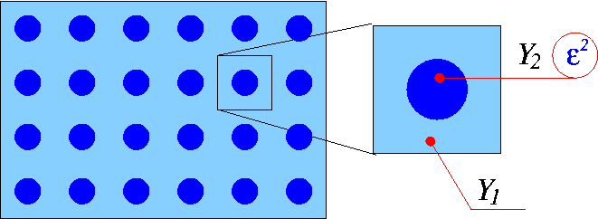
Periodic structure of the piezoelectric composite with $\veps^2$ -scaled material in the inclusions $Y_2$ .

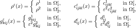
Properties of a piezoelectric material are described by three tensors: the elasticity tensor $c_{ijkl}^\veps$ , the dielectric tensor $d_{ij}^\veps$ and the piezoelectric coupling tensor $g_{kij}^\veps$ , where $i,j,k = 1,2,\dots,3$ .

We assume that inclusions are occupied by a very soft material in such a sense that there the material coefficients are significantly smaller than those of the matrix compartment, except the material density, which is comparable in both the compartments; as an important feature of the modelling, the strong heterogeneity is related to the geometrical scale of the underlying microstructure by coefficient $\veps^2$ :

$\begin{split} \rho^\veps(x) = \left \{ \begin{array}{ll} \rho^1 & \mbox{ in } \Om_1^\veps, \\ \rho^2 & \mbox{ in } \Om_2^\veps, \end{array} \right . & \quad \quad c_{ijkl}^\veps(x) = \left \{ \begin{array}{ll} c_{ijkl}^1 & \mbox{ in } \Om_1^\veps, \\ \veps^2 c_{ijkl}^2 & \mbox{ in } \Om_2^\veps, \end{array} \right . \\ g_{kij}^\veps(x) = \left \{ \begin{array}{ll} g_{kij}^1 & \mbox{ in } \Om_1^\veps, \\ \veps^2 g_{kij}^2 & \mbox{ in } \Om_2^\veps, \end{array} \right . & \quad \quad d_{ij}^\veps(x) = \left \{ \begin{array}{ll} d_{ij}^1 & \mbox{ in } \Om_1^\veps, \\ \veps^2 d_{ij}^2 & \mbox{ in } \Om_2^\veps. \end{array} \right . \end{split}$

Problem formulation¶

We consider a stationary wave propagation in the medium introduced above. For simplicity we restrict the model to the description of clamped structures loaded by volume forces and subject to volume distributed electric charges. For a synchronous harmonic excitation of a single frequency $\om$

$\tilde\fb(x,t) = \fb(x)e^{i\om t}\;, \quad \tilde{q}(x,t) = q(x) e^{i\om t}\;,$

where $\fb = (f_i),i=1,2,3$ is the magnitude field of the applied volume force and $q$ is the magnitude of the distributed volume charge, we have in general a dispersive piezoelectric field with magnitudes $(\ub^\veps,\vphi^\veps)$

$\tilde\ub^\veps(x,\om,t) = \ub^\veps(x,\om)e^{i\om t}\;, \quad \tilde{\vphi}^\veps(x,\om,t) = \vphi^\veps(x,\om) e^{i\om t}\;.$

This allows us to study the steady periodic response of the medium, as characterized by fields $(\ub^\veps,\vphi^\veps)$ which satisfy the following boundary value problem:

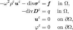
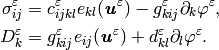
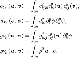
$\begin{split} -\om^2\rho^\veps \ub^\veps - \dvg \sigmabf^\veps & = \fb \quad \mbox{ in } \Om, \\ -\dvg \bmi{D}^\veps & = q \quad \mbox{ in } \Om,\\ \ub^\veps & = 0 \quad \mbox{ on } \pd\Om, \\ \vphi^\veps & = 0 \quad \mbox{ on } \pd\Om, \end{split}$

where the stress tensor $\sigmabf^\veps = (\sigma_{ij}^\veps)$ and the electric displacement $\bmi{D}^\veps$ are defined by constitutive laws

$\begin{split} \sigma_{ij}^\veps & = c_{ijkl}^\veps e_{kl}(\ub^\veps) - g_{kij}^\veps \pd_k \vphi^\veps, \\ D_k^\veps & = g_{kij}^\veps e_{ij}(\ub^\veps) + d_{kl}^\veps \pd_l \vphi^\veps. \end{split}$

The problem eq{eq-11} can be weakly formulated as follows: Find $(\ub^\veps,\vphi^\veps) \in \HOdb(\Om)\times \HOd(\Om)$ such that

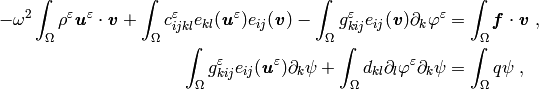
$\begin{split} -\om^2 \int_\Om \rho^\veps \ub^\veps \cdot \vb + \int_\Om c_{ijkl}^\veps e_{kl}(\ub^\veps) e_{ij}(\vb) - \int_\Om g_{kij}^\veps e_{ij}(\vb)\pd_k \vphi^\veps & = \int_\Om \fb\cdot\vb \;, \\ \int_\Om g_{kij}^\veps e_{ij}(\ub^\veps) \pd_k\psi + \int_\Om d_{kl}\pd_l\vphi^\veps \pd_k\psi & = \int_\Om q \psi \;, \end{split}$

for all 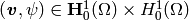$(\vb,\psi) \in \HOdb(\Om)\times\HOd(\Om)$ , where $\fb \in \Lb^2(\Om)$ , $q \in L^2(\Om)$ .

Spectral problem¶

Let us denote

$\begin{split} \aY2{\ub}{\vb} & = \int_{Y_2} c_{ijkl}^2 e_{kl}^y(\ub)\,e_{ij}^y(\vb),\\ \dY2{\phi}{\psi} & = \int_{Y_2} d_{kl}^2 \pd_l^y \phi\,\pd_k^y \psi,\\ \gY2{\ub}{\psi} & = \int_{Y_2} g_{kij}^2 e_{ij}^y(\ub)\,\pd_k^y \psi,\\ \rY2{\ub}{\vb} & = \int_{Y_2} \rho^2 \ub \cdot \vb, \end{split}$

whereby analogical notation is used when integrating over $Y_1$ .

The spectral problem reads as: find eigenelements $[\lam^r; (\zb^r,p^r)]$ , where $\zb^r \in \HOdb(Y_2)$ and $p^r \in H_0^1(Y_2)$ , $r=1,2,\dots$ , such that

$\begin{split} \aY2{\zb^r}{\vb} - \gY2{\vb}{p^r} & = \lam^r \rY2{\zb^r}{\vb}\quad \forall \vb \in \HOdb(Y_2), \\ \gY2{\zb^r}{\psi} + \dY2{p^r}{\psi} & = 0 \quad \forall \psi \in H_0^1(Y_2), \end{split}$

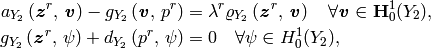
with the orthonormality condition imposed on eigenfunctions $\zb^r$ :

$\aY2{\zb^r}{\zb^s}+ \dY2{p^r}{p^s} & = \lam^r \rY2{\zb^r}{\zb^s} \stackrel{!}{=} \lam^r \delta_{rs}.$

Homogenized coefficients¶

The macroscopic model of elastic waves in strongly heterogeneous piezoelectric composite involves two groups of the homogenized material coefficients:

the homogenized coefficients depending on the incident wave frequency - these are responsible for the dispersive properties of the homogenized model. This group of the coefficients depends just on the material properties of the inclusion (except the material density, which is averaged over entire $Y$ )

the second group of coefficients is related exclusively to the matrix compartment – it determines the macroscopic piezo-elastic properties.

Let us summarize just the first group of coefficients, as those are connected with the appearance of the band gaps.

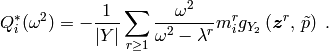
We introduce the eigenmomentum $\mb^r = (m_i^r)$ ,

$\mb^r = \int_{Y_2} \rho^2 \zb^r.$

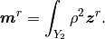
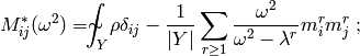
Then the following tensors are introduced, all depending on $\om^2$ : - Mass tensor $\Mb^* = (M_{ij}^*)$

$M_{ij}^*(\om^2) = \intYi{}\rho \delta_{ij} - \frac{1}{|Y|}\sum_{r \geq 1} \frac{\om^2}{\om^2 - \lam^r} m_i^r m_j^r\;;$

Applied load tensor $\Bb^* = (B_{ij}^*)$

$B_{ij}^*(\om^2) = \delta_{ij} - \frac{1}{|Y|}\sum_{r \geq 1} \frac{\om^2}{\om^2 - \lam^r} m_i^r \int_{Y_2} z_j^r\;;$

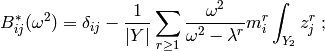
Applied charge tensor $\Qb^* = (Q_{i}^*)$

$Q_i^*(\om^2) = - \frac{1}{|Y|}\sum_{r \geq 1} \frac{\om^2}{\om^2 - \lam^r} m_i^r \gY2{\zb^r}{\tilde{p}}\;.$

Band gaps¶

The band gaps are frequency intervals for which the propagation of waves in the structure is disabled or restricted in the polarization.

The band gaps can be classified w.r.t. the polarization of waves which cannot propagate. Given a frequency $\omega$ , there are three cases to be distinguished according to the signs of eigenvalues $\gamma^r(\om)$ , $r = 1,2,3$ (in 3D), which determine the ``positivity, or negativity’’ of the mass:

{bf propagation zone} – all eigenvalues of $M_{ij}^*(\omega)$ are positive: then homogenized model eq{eq-45s} admits wave propagation without any restriction of the wave polarization;

{bf strong band gap} – all eigenvalues of $M_{ij}^*(\omega)$ are negative: then homogenized model eq{eq-45s} does {it not} admit any wave propagation;

{bf weak band gap} – tensor $M_{ij}^*(\omega)$ is indefinite, i.e. there is at least one negative and one positive eigenvalue: then propagation is possible only for waves polarized in a manifold determined by eigenvectors associated with positive eigenvalues. In this case the notion of wave propagation has a local character, since the ``desired wave polarization’’ may depend on the local position in $\Om$ .

In Fig. Distribution of the band gaps. we illustrate weak band gap distribution for piezoelectric composite formed by matrix PZT5A with embedded spherical inclusions made of BaTiOx3.

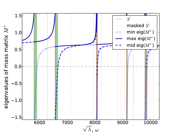
Distribution of the band gaps.

Distribution of the weak band gaps (white strips) for the piezoelectric composite. The curves correspond to eigenvalues of the mass tensor $\Mb^*(\om)$ .

The software can also perform dispersion analysis of long guided waves, a example result is shown in Fig. The dispersion analysis..

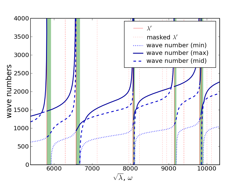
The dispersion analysis.

Illustration of the dispersion analysis output for the piezoelectric composite, angle of incidence is 45 $\deg$ . In the weak band gaps (grey/green strips) analyzed according to Fig. Distribution of the band gaps. waves can propagate in one or two directions only. In the second band gap only one polarization exists, with the phase velocity determined by the blue (solid) curve, in the first band gap two polarizations can propagate. In the ``full propagation zones’’ (white) the three curves correspond to the three wave polarizations.}

References¶

[rohan-miara-seifrt-2009]

Rohan, E., Miara, B. and Seifrt, F., 2009. Numerical simulation of acoustic band gaps in homogenized elastic compo sites. International Journal of Engineering Science. 4(47):573-594. doi://10.1016/j.ijengsci.2008.12.003.

Running a simulation¶

The band gap related problems can be solved by running the eigen.py script:

Usage: eigen.py [options] filename_in

Options:
  --version         show program's version number and exit
  -h, --help        show this help message and exit
  -o filename       basename of output file(s) [default: <basename of input
                    file>]
  -b, --band-gaps   detect frequency band gaps
  -d, --dispersion  analyze dispersion properties (low frequency domain)
  -p, --plot        plot frequency band gaps, assumes -b
  --phase-velocity  compute phase velocity (frequency-independet mass only)

Above filename_in stands for one of the problem definition files listed below. Each of the files contains all the necessary information to compute acoustic band gaps (ABG) and/or dispersion properties (DP) , namely:

band_gaps.py (ABG + DP in elastic material)

band_gaps_liquid.py (ABG in elastic material with fluid-like inclusion)

band_gaps_piezo.py (ABG + DP in piezoelastic material)

band_gaps_rigid.py (ABG in elastic material with rigid inclusion)

Each of the above files includes further options, that can be set to influence both the computation and subsequent postprocessing of results (accuracy settings, names and format of result files etc.).

Postprocessing¶

Results of a simulation are:

graphical representation of ABG and eventually DP; the figure are saved to the directory specified in options of each problem definition file,

text file of ABG, DP logs for custom postprocessing using plot_gaps.py script,

eigenfunctions of the related elasticity or piezoelasticity eigenvalue problems in the standard VTK format or a custom HDF5-based format, eigenvalues in text files.

User’s Guide¶

Introduction¶

Strongly heterogeneous material¶

Problem formulation¶

Spectral problem¶

Homogenized coefficients¶

Band gaps¶

References¶

Running a simulation¶

Postprocessing¶

Table Of Contents

Previous topic

Next topic

This Page

Navigation

User’s Guide¶

Introduction¶

Strongly heterogeneous material¶

Problem formulation¶

Spectral problem¶

Homogenized coefficients¶

Band gaps¶

References¶

Running a simulation¶

Postprocessing¶

Table Of Contents

Previous topic

Next topic

This Page

Quick search

Navigation